The Framework of Reality

For centuries, humanity has sought to understand the true nature of reality. Science and philosophy have attempted to describe the fundamental structure of the universe, yet contradictions, paradoxes, and unresolved anomalies have persisted.

The Dimensional Memorandum Framework is the missing key—a unification that integrates physics, cosmology, quantum mechanics, consciousness, propulsion, medical advancements, and energy technologies into a single, coherent model. It provides structured explanations for the Big Bang, black holes, quantum entanglement, dark matter, dark energy, and even the fundamental nature of time, perception, and technological advancements.

The Dimensional Memorandum Framework (DM)

We restore simplicity by showing that all scales, from quantum to cosmic, are governed by the same geometry.

Explaining why multiple "unrelated" anomalies share the same root. Replacing assumptions with a single geometric invariant.

Before introducing any new framework, it is important to recognize a fact that is often overlooked:

The Constants of Nature Are the Structural Fingerprints of Reality

In modern SI units:

• The speed of light c and Planck’s constant h are defined exactly.

• Electrical standards (K_J, R_K, Φ₀) are algebraically fixed by h and e.

• Vacuum constants (μ₀, ε₀, Z₀) are functions of c and the fine-structure constant α.

• Planck units are generated from {c, ħ, G}.

The apparent “zoo” of constants already collapses into a small dependency graph. What DM offers here, is a unifying geometric explanation of why collapse exists and where each constant sits in the structure of reality.

Planck units arise as natural endpoints:

• Planck length ℓₚ: minimum spatial resolution.

• Planck time tₚ: minimum temporal interval.

• Planck frequency ƒₚ = 1/tₚ: maximum meaningful rate.

While Planck’s constant ħ is the conversion factor between phase frequency and energy:

E = ħ ω

The One Invariant

R(s) f(s) = c

Expansion along one axis is exactly conjugate to contraction along the dual axis. It is a 45° slope invariant in log-space.

The ladder:

R(s) = ℓₚ e^{+s/λₛ}

ƒ(s) = ƒₚ e^{-s/λₛ}

Multiply:

R(s) ƒ(s) = ℓₚ ƒₚ = c

Collapse ħ:

E = ħ ω

E = m c²

So:

m = ħ ω / c²

Using ω = c / R:

m = ħ / (c R)

Mass is curvature created by projecting frequency into space. ħ fixes the conversion between rotation and extension.

Collapse G:

rₛ = 2Gm / c²

Substitute m:

rₛ = (2G / c²) (ħ / (cR))

Solve:

G = c³ R rₛ/ (2ħ)

At Planck scale:

R ≈ rₛ ≈ ℓₚ

So:

G = c³ ℓₚ² / ħ

G is a curvature conversion factor imposed by projection depth.

Collapse k_B:

E = k_B T

E = ħ ω

So:

k_B = ħ ω / T

Temperature is statistical spread in frequency.

Collapse Λ:

ρ_Λ ≈ Λ c² / (8πG)

ρ ≈ m / R³ ≈ ħ / (c R⁴)

So:

Λ ≈ 1 / R²

At cosmic scale:

Λ ≈ ℓₚ⁻² e^{-2s/λₛ}

The 10¹²² gap is simply:

(e¹⁴⁰)²

All constants are artifacts of projecting a higher-dimensional invariant onto lower-dimensional perception.

Quantum mechanics occupies the midpoint, where spatial localization and temporal coherence are balanced (near Compton frequencies ~10²⁰–10²⁴ Hz).

Starting with

Equilibrium

As physical systems project away from the Planck-scale into extended spacetime, two opposing processes occur simultaneously. Coherence decays with increasing dimensional depth, while spatial extent expands by the same geometric measure. These processes are not independent; they are symmetry-locked such that their product remains invariant. The invariant value of this product defines the speed of light.

The Coherence–Expansion Equilibrium:
c = R(s) · ƒ(s)

The coherence frequency decays exponentially with depth:
ƒ(s) = ƒₚ · e^(−s / λₛ)

The corresponding spatial scale expands exponentially:
R(s) = ℓₚ · e^(+s / λₛ)

Here, ƒₚ is the Planck frequency, ℓₚ is the Planck length, and λₛ is the coherence decay length. The speed of light is the invariant equilibrium between expanding spatial extent and collapsing coherence frequency:

ℓₚ ƒₚ = c

Space expands upward in scale. Frequency collapses downward. Their product remains fixed.

dR/ds = R/λₛ\n

Conjugacy Between Expansion and Contraction

3D R · ƒ = c Classical causality and localization (ρ)

R(s) = ℓₚ e^{+s/λₛ}
ƒ(s) = ƒₚ e^{−s/λₛ}

Invariant:
R(s) · ƒ(s) = ℓₚ ƒₚ = c

4D m · t = ħ / c² Wave propagation and quantum phase (Ψ)

m(s) = mₚ e^{−s/λₛ}
t(s) = tₚ e^{+s/λₛ}

Invariant:
m(s) · t(s) = mₚ tₚ = ħ / c²

5D G · ρ · t² / c² ≈ 1 Curvature / gravity and coherence stabilization (Φ)

ρ(s) = m(s) / R(s)³

Planck-normalized invariant:
G · ρ(s) · t(s)² / c² ≈ 1

Preserving ℓₚ ƒₚ = c:

ℓₚ = c tₚ

mₚ tₚ = ħ / c²

tₚ² = ħ G / c⁵

The Coherence–Expansion Equilibrium demonstrates that the speed of light arises as a fixed point between two exponential geometric processes. Coherence decays. Space expands. Their product remains constant.

Balance (+s/λₛ) ⇄ (-s/λₛ)

There is an opposition between localized physics and entangled coherence, with quantum occupying the unique midpoint where mass, space, time, and frequency are balanced. mt = h/c²

Below the balance: spatial extension dominates while frequency and mass contract: R(s) large, ƒ(s) small (m↓ - t↑)
The invariant R(s) · ƒ(s) = c ensures causal consistency. Localization arises because frequency is low enough to permit stable spatial embedding. Classical objects, trajectories, and deterministic causality emerge in this regime. This produces localized objects, classical trajectories and separable systems.

Balance: conjugate quantities start balancing where m(s) · t(s) = ħ / c². Here, mass, time, phase and energy are equal partners:

• Compton Wavelength / Frequency λ_C = ħ/(mc), ƒ_C = mc²/h (10²⁰-10²⁵):

Below 10²⁰ physics appears classical; above 10²⁵ localization fails.

• Rest Mass Energy (mc²): Pure conversion factor between frequency and inertia. It is neither kinetic nor gravitational, but the equilibrium exchange rate between time, energy, and mass.

• Quantum Phase exp(−iEt/ħ): Phase is neither energy nor time but their ratio. It exists only when mass and time are geometrically equivalent.

Here mass behaves like time, time behaves like space, wave propagation is stable, and both localization and coherence coexist.

Outside of this midpoint (R=ƒ), systems become either fully localized below (R↑-ƒ↓) or fully delocalized above (R↓-ƒ↑).

The exact midpoint 10²⁴ (c³), is also the turning point. Above this localization fails. The last seen particle is at 10²⁵ Hz, because particles cease to be well defined above this point. Which is why LHC sees null results beyond 10²⁵-10²⁷ Hz.

Above the balance: frequency and mass dominate while spatial localization fails: ƒ(s) large, R(s) small (m↑-t↓). The same invariant R(s) · ƒ(s) = c holds, but spatial coordinates lose meaning. States are no longer localized; instead, they are coherent across extended regions of Φ. Locality collapses, separation becomes irrelevant and systems behave as a single object. This is the geometric origin of quantum entanglement and nonlocal correlations. It also identifies why gravity does not need to be quantized in the usual sense.

Frequency band: 10²⁵ Hz → 10³² Hz

RG analogue: The regime where effective field theories reorganize into operator-dominated descriptions, governed by scaling dimensions, universality, and approach to UV control rather than new particle content.

Holography analogue: The boundary-to-bulk radial lift where boundary data begins reconstructing bulk geometry in AdS/CFT.

Λ Hierarchy (Full Projection Gap)

The Λ hierarchy is the full projection from boundary-accessible physics to Planck-scale closure across the s‑depth of the coherence field. It manifests as the observed ~10¹²² hierarchy in vacuum energy, entropy, and curvature.

Frequency span: 10²⁵ Hz → 10⁴³ Hz

Equivalent scan relation:
(ƒₚ / H₀)² ≈ 10¹²², with ƒₚ ≈ 10⁴³ Hz and H₀ ≈ 10⁻¹⁸ s⁻¹

RG analogue: The cosmological constant problem, interpreted as an IR/UV hierarchy where vacuum energy is naturally UV‑scale but observed only as a deeply IR-suppressed quantity.

Holography analogue: The Bekenstein–Hawking entropy hierarchy and area law, where bulk gravitational strength reflects an enormous number of boundary degrees of freedom.

Dimensional Clarity with DM

DM Explains Constants Geometrically

The fine-structure constant (α), proton–electron ratio (μ), Bohr radius, Rydberg constant, and more are outputs, not inputs.

c = ℓₚ / tₚ

ħ = Eₚ / ωₚ
G = c⁵/(ħ ƒₚ²)
α = exp(−ε) with ε = −ln(Z₀/120π)
H₀ = ƒₚ 10⁻⁶¹
Λ = (H₀/c)²
δ_CMB = √(H₀/ƒₚ)

Matching all simultaneously.

The Cosmological Constant problem:

Quantum field theory predicts Λ_QFT ≈10¹²² Λ_obs.
DM resolves this through geometric scaling:
(ƒₚ / H₀)² = 10¹²²
And predicts the observed CMB RMS anisotropy:
δ = √(H₀/ƒₚ) ≈ 10⁻⁵

This provides a direct analytic resolution, reproducing both the Λ-gap and the observed CMB anisotropy amplitude without parameter tuning.

DM Supplies a Universal Frequency Spectrum

A ladder from biological rhythms (Hz) to qubits (GHz), to particle rest frequencies (~10²³ Hz), to the Higgs (~10²⁵ Hz), and up to the Planck frequency (~10⁴³ Hz).

Connects seamlessly:

Orbital capacities (2, 6, 10, 14) emerge from B₄ reflection symmetry. Chemical frequencies inhabit 10¹⁵–10²⁰ Hz. Particle masses cluster at 10²³–10²⁵ Hz. Cosmological scaling spans 10⁻¹⁸→10⁴³ Hz. Dark energy matches Φ slow-beat.

DM provides a single geometric architectural that simultaneously accounts for constants, scaling, and structure across quantum, atomic, and cosmological regimes.

Links Quantum, Relativity, and Cosmology Using First Principles

The sequence B₃ → B₄ → B₅ precisely maps to the evolution of localized matter (ρ), time (Ψ), and coherence (Φ), corresponding respectively to classical mechanics, wave–spacetime, and coherence-stabilized fields.
The Coxeter Bₙ sequence defines the discrete reflection symmetries underlying reality’s geometry. Each dimensional expansion adds an orthogonal axis of movement, transforming static geometry into dynamic physical law.

1. First Principles Cascade

Each expansion adds an orthogonal degree of freedom:
B₃(x,y,z) → B₄(x,y,z,t) → B₅(x,y,z,t,s). All information stored on boundaries B₅→B₄→B₃→B₂

3D Cube ρ

(face 10⁰-10¹² Hz)

sub-c¹ ≈ 10⁰ → 10⁷ Point in time

Perceptual time at face:

c¹ ≈ 10⁸ → 10¹⁵ Line in time

Movement from point to point (sub-c¹) in a line (c¹).

True geometric face:

c² ≈ 10¹⁶ → 10²³ Squared time (area)

The cross-section of 4D, experienced in 2D frames. Rate ≈ 1 / tₚ ≈ 1.85 × 10⁴³ waves (frames) per second.

3D data exhausts at 10²³

Classical Physics

x,y,z with planar surfaces (info)

4D Tesseract Ψ

(face 10²³-10²⁷ Hz)

sub-c¹ ≈ 10⁰ → 10⁷ Point

c¹ ≈ 10⁸ → 10¹⁵ Lined

Perceptual time at face:

c² ≈ 10¹⁶ → 10²³ Squared time (area)

m, t, h, E equal out. R = ƒ.

Particle rest-mass. Mid-point

True geometric face:

c³ ≈ 10²⁴ → 10³¹ Cubed (volume)

Volume (c³) of areas (c²) = overlapping waves.

Time-space flips (10²⁴). Horizon begins (10²⁵).

4D data exhausts at 10³²

Quantum Mechanics

x,y,z,t with volume surfaces (info)

5D Penteract Φ

(face 10³³-10⁴³ Hz)

0D: sub-c¹ ≈ 10⁰ → 10⁷ Point

1D: c¹ ≈ 10⁸ → 10¹⁵ Lined

2D: c² ≈ 10¹⁶ → 10²³ Squared

3D: c³ ≈ 10²⁴ → 10³¹ Cube

Geometric face:

4D: c⁴ ≈ 10³² → 10³⁹ Tesseract

Full space/time hypervolume (bulk)

5D: c⁵ ≈ 10⁴⁰ → 10⁴³ Penteract (10 bulks)

Pₚ = c⁵/G; Planck force: Fₚ = c⁴/G; tₚ, ℓₚ, ƒₚ. Eₚ = h ƒₚ. Planck scan: c = ℓₚ / tₚ.

Coherence Field

x,y,z,t,s with hypervolume surfaces (info)

1.2 (A) Boundary Sampling

A D-dimensional observer can only access information encoded on (D−1)-dimensional hypersurfaces. This principle follows from causal structure, holography, and entropy bounds, and is a geometric necessity.

Information accessible to an observer is restricted to codimension-1 boundaries:
I_obs ∝ ∂(Geometry)
A 3D observer samples 2D surfaces

The Bekenstein–Hawking entropy law:
S = A / (4 ℓₚ²)
demonstrates that gravitational systems encode information in area, not volume.

Observed information arises from boundary integrals:
I_D(x) = ∫_{Σᴰ⁻¹} Φ(x, ξ) dᴰ⁻¹ξ
Thus, 3D observers integrate over 2D faces of higher-dimensional fields.

Relation to Time and Causality

Time acts as an ordering parameter. Motion through higher-dimensional geometry manifests as temporal evolution on lower-dimensional faces.

Information propagates face-to-face across dimensions:
5D → 4D faces = fields (hyper-volumes)
4D → 3D faces = waves (volumes)
3D → 2D faces = localized objects (areas)

A D-dimensional observer can only access information encoded on (D−1)-dimensional hypersurfaces because causal propagation restricts measurement to codimension-1 boundaries.

1.2 (B) Resolution of the Measurement Problem

A 3D observer cannot access a full 4D quantum object and instead samples only lower-dimensional boundary surfaces. What appears as wavefunction collapse is the geometric projection of a higher-dimensional coherent object onto a lower-dimensional boundary. This resolves collapse, discreteness, irreversibility, and nonlocal correlations without introducing hidden variables, observer-dependent dynamics, or modifications to quantum mechanics

In any dimensional hierarchy, an observer embedded in D dimensions cannot directly access the full interior of a D+1 dimensional object. Instead, information is obtained through boundary intersections. This is a geometric fact, not a physical assumption.

Formalized as a boundary sampling operation:

I_D(x) = ∫_{Σ^{D−1}} Φ(x, ξ) d^{D−1}ξ

This operation is neither unitary nor time-evolutionary; it is a projection imposed by dimensional limitation.

Collapse Along the s-Axis (5D → 4D)
The coherence field Φ(x,y,z,t,s) exists in five dimensions. Direct observation of s is impossible for 4D observers. The effective 4D wavefunction arises from projection along the s-axis:

Ψ(x,y,z,t) = ∫₀^∞ Φ(x,y,z,t,s) e^(−s/λₛ) ds ≈ Φ λₛ
This projection reduces the available degrees of freedom by one, corresponding to the reduction from B₅ symmetry to B₄ symmetry. The associated entropy scaling shifts from ~10¹²² to ~10¹²¹, reflecting the loss of one geometric axis.

Collapse Along the t-Axis (4D → 3D)
A 3D observer does not experience time volumetrically. Instead, time is sampled as a cross-section. This produces the apparent localization of quantum states:

ρ(x,y,z,t₀) = ∫ Ψ(x,y,z,t) δ(t − t₀) dt = Ψ(x,y,z,t₀)
This is the true origin of wavefunction collapse. The wave does not disappear; rather, the observer samples a fixed temporal slice. The reduction B₄ → B₃ corresponds to a further entropy compression from ~10¹²¹ to ~10⁶¹.

Why Collapse Appears Non-Unitary
Unitary evolution governs dynamics within a fixed dimensional space. Boundary sampling is not evolution but dimensional projection. As such, it is inherently irreversible and non-unitary. No modification of quantum mechanics is required.

Discreteness, Probability, and the Born Rule
Measurement outcomes appear discrete because boundary surfaces have finite area. The Born rule emerges naturally as a surface measure over Σ². Probabilities correspond to relative surface intersections, not intrinsic randomness

Resolution of the Measurement Problem
All standard features of quantum measurement follow directly from boundary sampling:
• Apparent collapse arises from dimensional projection
• Irreversibility follows from information loss
• Discreteness follows from finite boundary area
• Nonlocal correlations follow from shared coherence
• No observer-dependent physics is required

The quantum measurement problem is resolved once measurement is recognized as a geometric boundary sampling process. A 3D observer necessarily collapses 4D coherence into localized outcomes because only lower-dimensional surfaces are accessible. This framework unifies quantum measurement with holography, renormalization, and gravitational entropy without altering established physics.

1.2 (C) Face-Storage (Boundary/Surface Encoding)

Physical observables in (n−1) dimensions are boundary functionals of n-dimensional fields:

Oₙ₋₁ = G[ Φₙ |_{∂Mⁿ} ]

Flux / Stokes Boundary Encoding

For any conserved current J in an n-dimensional manifold M^(n):
∫_{Mⁿ} dⁿ x ∇·J = ∫_{∂Mⁿ} dⁿ⁻¹Σ (J · n̂)
If ∇·J = 0, all observable information transfer occurs through the boundary.

Variational Boundary Encoding (GR/QFT)

The action requires explicit boundary terms:
S = ∫_{Mⁿ} L dⁿ x + ∫_{∂Mⁿ} B dⁿ⁻¹x

In General Relativity:
S_EH = (1/16πG) ∫ √−g R d⁴x + (1/8πG) ∫ √|h| K d³x
The boundary term encodes the data necessary for bulk evolution.

Entropy / Holographic Bound

Maximum information content scales with boundary area:
S_max ≤ k_B A / (4 ℓₚ²)

Generalized to n dimensions:
log N_states ∝ Area(∂Mⁿ) / ℓₚⁿ⁻²

DM Projection-to-Face Formulation

3D observables are time-slices of 4D wavefunctions:
ρ(x,y,z) = ∫ Ψ(x,y,z,t) δ(t − t0) dt
4D wavefunctions are boundary projections of 5D coherence fields:
Ψ(x,y,z,t) = ∫ Φ(x,y,z,t,s) w(s) ds

Thus:
Φₙ₋₁ = Φₙ |_{∂Mⁿ

Rindler horizons

Introducing Rindler coordinates (η, ξ), the Minkowski metric becomes:
ds² = −(aξ)² dη² + dξ² + dy² + dz².
The surface ξ = 0 defines a causal horizon. This horizon arises without spacetime curvature, purely from the observer’s kinematic slicing of spacetime.

At the Rindler horizon (ξ → 0), the metric coefficient g_ηη → 0. The observer-adapted time coordinate degenerates, mirroring the behavior of Schwarzschild time at a black hole event horizon.

Upon Wick rotation (η → iη_E), the Rindler metric becomes locally polar near the horizon. Regularity requires η_E to be periodic with period:
Δη_E = 2π / a.
This periodicity implies a thermal state with temperature:
T_U = ħ a / (2π c k_B).
Thermality is a geometric consequence of horizon-adapted coordinates, not a dynamical particle-creation process.

Equivalence with Black Hole Thermodynamics

Hawking temperature for a black hole is given by:
T_H = ħ κ / (2π c k_B), where κ is the surface gravity at the event horizon. The Unruh and Hawking effects are mathematically identical, differing only in whether the horizon arises from acceleration or spacetime curvature.

Horizons correspond to projection boundaries between dimensional domains. Observers access only a boundary ‘face’ of the full geometric structure. Degrees of freedom beyond the horizon are effectively traced out, converting pure states into mixed states and producing entropy and temperature.

Across physics, information is encoded on lower-dimensional faces. This is a direct consequence of conservation laws, variational principles, entropy bounds, and dimensional projection.

1.3 Projection Channels (Hz)

Einstein–Coherence equation:

G_{μν} + S_{μν} = (8πG/c⁴)(T_{μν} + T^{(Φ)}_{μν}) + Λₛ e^{−s/λₛ} g_{μν}

Λₛ e^{−s/λₛ} g_{μν} (Projection Envelope)

Standard GR is recovered by taking the classical projection limit:
• s → ∞ (deep projection)
• ∂_s Φ → 0 (no coherence gradients)
• T^{(Φ)}_{μν} → 0 (bulk coherence unobservable)

Under these conditions:
S_{μν} → 0
Λₛ e^{−s/λₛ} → Λ (constant)

The equation reduces exactly to:
G_{μν} = (8πG/c⁴) T_{μν} + Λ g_{μν}
which is the Einstein field equation with cosmological constant.

Dominant:

Classical

Quantum

Field

t↑-m↓

Exhaustion of 3D info

t↓-m↑

Higgs

c⁵

c⁴

c³

c²

c¹

sub-c¹

10⁴⁰

10³²

10¹⁶

10⁸

10²⁴

10⁴³

x,y,z,t,s

x,y,z,t

x,y,z

x,y

Horizon begins

Chemistry ends

Exhaustion of 4D info

Time←

→Space

Planck ceiling: ƒₚ ⇒ S ≈ 10⁸⁶

Flip

Electron Rest-Mass, plus:

10²⁰–10²² Hz: e⁻, ν, quarks

10²²–10²⁴ Hz: μ, τ, p/n

10²⁵ Hz: W, Z, H

Fully local to time

Fully non-local

point

lined

squared

cube

tesseract

penteract

c = ℓₚ / tₚ

m · t = ħ / c²

G_{μν}

G = c³ ℓₚ² / ħ

Holographic principle is exact here.

volume → bulk

E = ħω

α = e^(−ε)

Z₀/120π^(−ε)

m = ħω / c²

Λ ~ 1/R²

tₚ, ℓₚ, ƒₚ, Eₚ, Fₚ, Pₚ

(10²⁵) Λ-gap begins

Λ-gap continues

E = k_BT = ħω

(wherever Ψ is)

Constants →

10²⁵→10³² Hz corresponds to the Ψ→Φ lift (loss of particle eigenstates and transition to operator language), while 10²⁵→10⁴³ Hz corresponds to the Λ hierarchy (full projection across s‑depth to Planck closure), whose entropy and counting expressions yield the observed ~10¹²² separation.

Between approximately 10³³ and 10³⁹ Hz, the system occupies a mixed-dimensional regime. Four-dimensional curvature channels remain active, while five-dimensional coherence gradients have already turned on:

∂ₛΦ ∼ α(f) · ∂_μΦ , 0 < α(f) < 1

Threshold (~10⁴⁰ Hz): ∂ₛΦ ⟂ ∂_μΦ. Above this, the system resides in a fully five-dimensional regime. All five axes (x, y, z, t, s) are independent. This regime naturally hosts:

• Black hole interiors
• Big Bang coherence states
• Topological and entropic invariants
• Planck-scale scan closure

Global coherence: Λ(s) = Λₛ e^(−2s/λₛ) 10⁻¹⁸ ⇆ 10⁴³

Operators

Field entry: 10²⁵

Dominant: 10²⁸

Exhaustion: 10³²

Organic

Chemistry

Rest-mass

LHC decay

S_{μν}

Black Holes

Stellar: ~10³³–10³⁵ Hz

~10¹–10² M☉

SMBH: ~10³¹–10³³

~10⁶–10¹⁰ M☉

Planck BH: ~10⁴³

mₚ

Big Bang

Black hole interiors ⇒

∇²Φ = 4πGρ

E² = (pc)² + (mc²)²

EM Light Spectrum

10⁶–10¹¹ Radio to Microwave

10¹²–10¹⁴ Infrared

≈4×10¹⁴–7×10¹⁴ Visible Light

10¹⁵–10¹⁸ Ultraviolet to X-rays

10¹⁹–10²³ Gamma Rays

10²⁴ γ‑ray cutoff

2. Simplicity and Unification

By reducing all of physics to pure geometry, DM achieves unification — where constants, forces, and particles are faces of a single structure. DM represents the transition from descriptive observation to geometric inevitability. This marks the era where Coherence becomes engineering.

2.1 Geometry and Algebra

The geometric nesting relationships between the symmetries (Bₙ) and algebra (Clₙ), demonstrates how each Coxeter reflection symmetry corresponds to a Clifford operator space one degree lower, defining the physical domain, operator behavior, and frequency partition of the universe.

Coxeter Symmetry (Bₙ)

Differential Operators

Clifford Algebra

(Clₙ)

Physical Role

Description

ρ 3D

B₃ – Cube / Octahedron

(48 elements)

∇, ∇·, ∇×

Cl₂ = {1, e₁, e₂, e₁e₂}

Electromagnetism /

spatial charge fields

Bivector rotations → E & B fields; 3D localized classical domain.

Ψ 4D

B₄ – Tesseract

(384 elements)

∇_μ, ∂_t

Cl₃ = {1, e₁, e₂, e₃, e₁e₂, e₂e₃, e₃e₁, e₁e₂e₃}

Spinor / wavefunction propagation

Dirac γ-matrices realize Cl₃ algebra, producing fermionic spinor structure in 4D.

Φ 5D

B₅ – Penteract

(3840 elements)

∇_μ, ∂_s

Cl₄ / Cl₅ – adds e₄

(or e₅)

Coherence field / curvature stabilization

Adds generator Γ⁵ (γ⁵); Spin(5) symmetry stabilizes divergences and curvature coupling.

2.2 Dimensional Frequency Relation

Each Clifford domain aligns with a distinct frequency partition defined by the exponential scaling law:

ƒₙ = ƒₚ · e^{−(n−2)Δs / λₛ}, with Clₙ ∼ Bₙ₊₁

As coherence depth s increases, the active algebra transitions:
Cl₂ → Cl₃ → Cl₄ → Cl₅
following the same exponential partition that defines DM’s frequency shells:

B₃ → Cl₂

3D (ρ) localized

B₄ → Cl₃

4D (Ψ) quantum wave

B₅ → Cl₄/₅

5D (Φ) coherence field.

Each Clifford algebra resides one level below its corresponding Coxeter symmetry, governing the operator space of that geometric layer.

Resolution

3D Classical Physics:

Cube ρ(x, y, z)

Planck volumes:
N₃D ≈ V / ℓₚ³ ≈ 10¹⁸⁵

Planck length lₚ ≈ 10⁻³⁵ m

(B₃ symmetry)

Spin(3) ≅ SU(2)

10³ (micro scaling steps)

~10⁶¹ (linear scaling steps)

1–10¹⁴ Hz

(biological/classical → decoherence thresholds)

ρ(x, y, z) = ∫ Ψ(x, y, z, t) · δ(t - t₀) dt

Frames / Waves

4D Quantum Mechanics:

Tesseract Ψ(x, y, z, t)

Planck cells:
N₄D ≈ N₃D × (T / tₚ) ≈ 10¹⁸⁵ × 10⁶¹ ≈ 10²⁴⁶

Planck time tₚ ≈ 10⁻⁴⁴ s

(B₄ symmetry)
Spin(4) ≅ SU(2)ꮮ × SU(2)ꭱ

10⁶ (micro scaling steps)

~10¹²¹ (area, volume scaling)

face 10²³-10²⁷ Hz

(wavefunctions, hadrons, SM decays)

Ψ(x, y, z, t) = ∫ Φ(x, y, z, t, s) · e^(–s / λₛ) ds

Coherence Entrance

5D Coherence Field:

Penteract Φ(x, y, z, t, s)

Hypercells:
N₅D ≈ N₄D × 10¹²² ≈ 10²⁴⁶ × 10¹²² ≈ 10³⁶⁸

Planck energy Eₚ ≈ 10¹⁹ GeV

(B₅ symmetry)
Spin(5) ≅ Sp(2)
10¹⁰ (micro scaling steps)

~10¹²² (coherence depth, Λ gap)

face 10³³–10⁴³ Hz

(coherence fields, dark matter/energy, black holes, Big Bang)

Φ(x, y, z, t, s) = Φ₀ · e^(−s²/λₛ²)

Planck's constants naturally arise from the geometric scaling of 3D (ρ) cubes, 4D (Ψ) tesseracts, and 5D (Φ) penteracts. These constants define the resolution, scanning rate, and curvature relationships of reality's dimensional layers. These ratios also naturally appear in the observed clustering of particle properties.

LHC

Why null results above the Higgs scale are expected and experimentally consistent.

LHC dynamics are governed by intrinsic frequencies associated with mass–energy via:
ƒ = E / h

Key scales:
- Proton Compton frequency: ƒₚ ≈ 2.3 × 10²³ Hz
- Higgs mass (125 GeV): ƒ_H ≈ 3.0 × 10²⁵ Hz
- LHC hard scatterings: 10²⁴–10²⁶ Hz

The c³ Hinge and Particle Identity

The band around 10²⁴ Hz marks the c³ hinge. Below this, particles remain localized. Above it, excitation shifts from particles to fields and operators.

Beyond the Higgs scale, physics ceases to be particle-based and becomes geometry / coherence dominated → meaning the next advances require phase (coherence) control, not higher energy.

Ψ Tesseract Face (10²³-10²⁷ Hz)

Used

Beam energy / kinetic frequency

E = γmc² ⇒ ƒ = E/h 2.4 x 10²⁶ Hz

Internal particle identity anchored at 10²³ Hz

10²⁴

10²⁵

10²³

10²⁶

c³

10²⁷

Operator-dominated regime.

Above Higgs boundary

no stable particle localization.

Bulk geometry begins and fully dominates by 10³² Hz.

Higgs

E=mc² completion

area to volume

← →

≥ 10²⁷ Hz

Smooth RG flow

E = ħω,
with ω = 2πƒ

m = ħƒ / c²,
Schwarzschild

rₛ = 2Gm / c²

← IR

UV →

local←

→nonlocal

ending of info

on planar

boundaries

continued info

on volumetric

boundaries until 10³¹

start of info

on bulk

boundaries

← Inside

Fold

Outside →

Why the Higgs is the Last Particle

The Higgs boson sits at the Ψ→Φ overlap (~10²⁵ Hz). It is the final excitation that remains marginally particle-like.
Above this scale, localization fails and particle descriptions dissolve.

All major LHC results since 2012 support this structure:
- No new resonances beyond Higgs
- Smooth high-energy cross sections
- No evidence for SUSY

The LHC has already answered their questions. These are signatures of a dimensional transition, not missing physics.

The LHC probes the terminal boundary of particle physics. Beyond ~10²⁵ Hz, geometry and coherence replace particles. The Dimensional Memorandum explains why the Standard Model closes where it does.

Mirror Equation

ƒ(s) · ƒ(−s) = ƒₚ · H₀
is mathematically identical to a renormalization-group (RG) fixed-point condition.

RG Fixed Points (Standard Definition)

In Wilsonian renormalization group theory, a coupling g(μ) evolves with scale μ according to
β(g) = μ dg/dμ
A fixed point g* satisfies
β(g*) = 0

At this point, physics becomes scale-invariant: degrees of freedom neither localize nor delocalize further.

ƒ(s) ƒ(−s) = ƒₚ H₀
states that UV and IR scales are conjugate. Taking logarithms:
ln ƒ(s) + ln ƒ(−s) = ln ƒₚ + ln H₀
This defines a symmetric fixed point at s = 0, where
ƒ_* = √(fₚ H₀) ≈ 10²⁴ Hz (c³)

At this scale, RG flow stalls: neither UV nor IR dominance applies.

Identification with Wilsonian RG

RG energy scale μ ⇆ DM frequency ƒ(s)
RG flow parameter ln μ ⇆ DM depth s/λₛ
RG fixed point μ* ⇆ DM mirror frequency ƒ*

The Higgs scale sits at this fixed point, explaining why:
• particle identities cease above it
• couplings stop producing new states
• effective field theory replaces particle descriptions
• geometry takes over beyond this scale

Below the fixed point (ƒ < ƒ*):
• mass increases
• localization dominates
• chemistry and particles exist

Above the fixed point (ƒ > ƒ*):
• mass delocalizes
• couplings run to geometry
• holography and curvature dominate

The mirror equation enforces this bifurcation automatically.

Because the RG fixed point is already realized at the Higgs scale:
• no supersymmetry can appear above it
• no new particles can stabilize
• LHC null results are expected
• UV completion must be geometric, not particle-based

The DM mirror equation is not an analogy to RG fixed points — it is the fixed-point condition, expressed geometrically. RG flow, holography, and cosmological scaling all emerge as corollaries of the same invariant.

Lined

Point

Flip

(Hz) →

10⁸

10¹⁶

10⁴

10¹²

10x Bulk

10⁶¹

10¹²¹

10¹²²

Space→

←Time

10⁶⁰

(Scaling Steps) →

Area

Volume

Bulk

Mirror

Higgs

10²⁴ Hz

10³²

10⁴⁰

10⁴³

10³⁶

10²⁰

10²⁸

T_age / tₚ ≈ 4.35 × 10¹⁷ s / 5.39 × 10⁻⁴⁴ s ≈ 8 × 10⁶⁰

R_obs / lₚ ≈ 4.4 × 10²⁶ m / 1.61 × 10⁻³⁵ m ≈ 2.7 × 10⁶¹

The combined ratios (~10¹²¹ total plank cells) is effectively the volume of the 4D tesseract and the full Universe is ~10¹²² total Planck cells.

3D ρ info

4D Ψ info

5D Φ info

Static

t: Pure ordering

m: Negligible

Transport

t: Flowing

m: Bound matter

Standing

t: Metric

m: Atomic mass

Operator

t: Delocalized

m: Particle disillusion

Coherent

t: Distributed

m: Field mass

Pure

t: Absent

m: Geometric

∂_ν F^{νμ}=μ₀J^μ; c²=1/(μ₀ε₀)

EFT of classical EM + condensed matter

m = ħω/c²; ƒ_C=mc²/h; Zα controls relativistic chemistry

QED/QM; running α(μ) mild

null peakes fields/operators

heavy DOFs integrated out; match onto EFT coefficients

Bounds: S ≤ 2πER/(ħc)

area laws emerge

radial depth ⇆ RG scale; entropic bounds constrain EFT

ℓₚ ƒₚ = c; Eₚ=ħωₚ; curvature/entropy dominate

geometric closure

x, y

x, y. z

x, y, z, t

x, y, z, t, s

Slow ω: E=ħω small

coarse‑grained DOFs; μ very low (IR)

Localization ←

binding, emergent structure, symmetry breaking

→ Delocalization

unbinding,, dissolved identity, symmetry restoration

RG cross over

(-10⁵) IR endpoint

m↓ - t↑

m↑-t↓

Fusion

LHC

decay

UV endpoint (-10⁵)

10²³

10²⁵

E = ħω,
with ω = 2πƒ

m = ħƒ / c²,
Schwarzschild

rₛ = 2Gm / c²

The invariant R · ƒ = c enforces a mirror symmetry,

with EM and locality on one side and curvature
and nonlocality on the other. All known scale hierarchies—including the Λ-gap and
holographic entropy—emerge as manifestations of this single geometric ordering principle.

3. Dual-Scale Coherence Law

DM demonstrates that micro-scale and cosmic-scale domains are geometrically linked through a single exponential coherence law. The relation ƒ(s) = ƒₚ e^{−s/λₛ} and Δx(s) = ℓₚ e^{s/λₛ} defines how frequencies and spatial scales expand or contract exponentially across dimensional depth s. Each domain in 3D (ρ) has a corresponding dual domain in 5D (Φ), and their product remains constant at approximately 10¹²², the cosmological Λ-gap ratio.

3.1 Exponential Coherence

The scaling principle of DM is:
ƒ(s) = ƒₚ e^{−s/λₛ}, Δx(s) = ℓₚ e^{s/λₛ}.

Each step in s/λₛ corresponds to a logarithmic scale change of 10ⁿ. The coherence depth Δs/λₛ = ln(10ⁿ) defines how geometry transitions between physical domains.

3.2 Micro–Macro Duality

• 10³ → mechanical oscillations and acoustic motion (localized ρ-domain).

Dual 10⁶¹ → gravitational-wave curvature amplitude (Φ-field).
• 10⁶ → biological resonance and cell-scale coherence.

Dual 10¹²¹ → dark energy curvature density.
• 10¹⁰ → atomic-scale electromagnetic field frequencies.

Dual 10¹²² → Λ-gap terminal ratio between Planck and cosmic horizons.

Each micro-level phenomenon is a projection of its macro-level coherence partner across the ρ–Ψ–Φ dimensional hierarchy.

3.3 Relation
10ᵐᶦᶜʳᵒ × 10ᵐᵃᶜʳᵒ = 10¹²² = e^{s_Λ / λₛ}
preserving the coherence invariant ƒ·Δx = c across all scales.

The paired exponents (10³–10⁶–10¹⁰) and (10⁶¹–10¹²¹–10¹²²) form the two faces of the Λ-gap. Their symmetry demonstrates that micro-scale phenomena and cosmic-scale curvature follow the same exponential law of coherence geometry. Relativistic effects, quantum frequencies, and cosmological constants are all unified through this dual-scale coherence law.

Mass, Time and Energy

3.4 Mass

Exponential coherence scaling applies uniformly to spatial extent, time, frequency, and mass.

Coherence Scaling relations:

R(s) = ℓₚ e^{+s/λₛ}
t(s) = tₚ e^{+s/λₛ}
ƒ(s) = ƒₚ e^{−s/λₛ}

Energy–Mass relation:

E(s) = h ƒ(s)
m(s) = E(s) / c²

Substituting the frequency scaling yields:
m(s) = (h / c²) ƒₚ e^{−s/λₛ} ≡ mₚ e^{−s/λₛ}, where mₚ = h ƒₚ / c² is the Planck mass scale.

The coherence ladder satisfies the invariant relation:
R(s) ƒ(s) = ℓₚ ƒₚ = c, ensuring that spatial expansion and frequency decay remain exactly balanced. Mass therefore decreases exponentially with coherence depth, mirroring the frequency decay and providing a unified description of localization across scales.

Where s is coherence depth and λₛ is the same suppression factor that produces Λ/Λ_Planck ≈ 10¹²². Same exponential. Same geometry.

Mass is a projection of coherence frequency into observer-accessible spacetime. Larger spatial scales correspond to lower characteristic frequencies and thus lower mass–energy densities, while smaller scales correspond to higher frequencies and stronger localization. This places mass on equal geometric footing with space, time, and frequency.

3.5 Time–Mass Duality

Time and mass are exact conjugates under coherence scaling, enforced by quantum phase invariance

m(s) = mₚ · e^{−s/λₛ}
t(s) = tₚ · e^{+s/λₛ}
with invariant product:
m(s) · t(s) = h / c².

Mass contraction and time dilation are dual manifestations of the same geometric scaling.

Quantum phase for a free system is given by:
φ = E t / ħ = m c² t / ħ.
Phase must remain invariant under changes in coherence depth s. Therefore, the product m(s)·t(s) must be constant. Planck-scale normalization fixes this constant to h / c², yielding the stated exponential laws.

Mass represents localized coherence, while time represents expanded coherence. Their duality explains why clocks slow in strong gravitational or energetic environments without invoking additional dynamics.

Gravitational Time Dilation

In curved spacetime, effective coherence depth varies with gravitational potential. A local shift s → s + Δs produces time dilation:
t → t · e^{Δs/λₛ}, recovering the qualitative behavior of general relativistic clock slowing as a geometric projection effect.

3.6 Relation Between the Time–Mass Duality and E = mc²

The Dimensional Memorandum framework aligns exactly with Einstein’s mass–energy equivalence E = mc², without modification or reinterpretation.

Einstein’s relation
E = mc² is not merely a conversion formula, but a statement that mass and energy are the same physical quantity viewed through the causal scale set by c.

Mass scales with coherence depth s according to:
m(s) = mₚ · e^{−s/λₛ}
Substituting into Einstein’s relation yields:
E(s) = m(s)c² = mₚ c² · e^{−s/λₛ}
Thus, energy contracts exponentially with coherence depth.

Quantum phase is given by:
φ = E t / ħ
Phase must be invariant under changes in coherence depth. Therefore:
E(s) · t(s) = constant
Substituting the energy scaling forces the time law:
t(s) = tₚ · e^{+s/λₛ}

Using Planck normalization, the invariant becomes:
E(s) · t(s) = mₚ c² tₚ = h
This shows that energy–time phase invariance is preserved exactly.

Relations
E = mc²
E t = h
are not independent statements. They arise as complementary projections of a single scale-invariant geometry:
• c² converts mass into energy at the causal boundary
• t(s) converts energy into quantum phase under coherence scaling

The Dimensional Memorandum preserves Einstein’s relation E = mc² exactly, while revealing why exponential mass scaling forces a conjugate exponential time law so that energy–phase invariance E(s)t(s) = h is maintained at all scales. The equivalence of mass and energy is thus not altered, but geometrically enforced.

Zitterbewegung and Standing Phase Mass

The Dirac equation for a free relativistic fermion is:
(iħγ^μ ∂_μ − mc)ψ = 0

The position operator exhibits rapid oscillatory motion (zitterbewegung) with angular frequency:

ω_z = 2mc² / ħ

This frequency corresponds to twice the Compton frequency, indicating intrinsic phase oscillation.

In DM, mass is identified with a stabilized standing phase at a projection boundary:
f_C = mc² / h
This frequency represents the equilibrium between spatial contraction and temporal oscillation.

The Planck Scan:
ℓₚ · fₚ = c

Relativistic Phase without Velocity

The Vienna TU experiments demonstrate Lorentz transformations as phase warping, not physical motion. DM models this as:
ψ(x,t) = A · exp[i(φ(x,t))] where φ evolves geometrically under projection.

Zitterbewegung arises from interference between forward and backward time components:
ψ = ψ₊ + ψ₋ with phase separation governed by coherence depth λₛ.

These equations show that mass, time, and phase are unified geometrically. Zitterbewegung is not anomalous but a necessary consequence of projection-stabilized phase.

3.8 Energy ladder

Coherence ladder (s-depth): ƒ(s) = ƒₚ e^(−s/λₛ), R(s) = ℓₚ e^(+s/λₛ)

Invariant (scan constraint): R(s) · ƒ(s) = ℓₚ ƒₚ = c

Quantum conversion: E = ħω = h ƒ

Rest-energy conversion: E = m c² ⇒ m = (h ƒ)/c² = (ħω)/c²

Compton relations: ƒ_C = m c² / h, λ_C = h/(m c)

Planck anchors: tₚ = √(ħG/c⁵), ℓₚ = √(ħG/c³), ƒₚ = 1/tₚ, Eₚ = h ƒₚ

Rung

Approx. Band (Hz)

Geometric Role

Primary Energy Form

Equations / Invariants (representative)

sub‑c¹

10⁰ → 10⁸

Point / event-time granularity (pre-transport)

Quasi-static energy; slow ordering / ‘clocking’

ƒ ≪ c/R → transport negligible; Δφ = 2π f Δt; E = h ƒ (tiny); thermodynamic/biological rhythms as low‑ƒ coherence

c¹

10⁸ → 10¹⁵

Line / causal transport regime (light-like communication dominates)

Radiative/propagating energy (photons, EM transport)

R f = c (transport bound); Maxwell waves: ω = c k; photon energy

c²

10¹⁶ → 10²³

Planar / squared-time regime (mass–time conjugacy operational)

Rest-energy and inertial energy bookkeeping

E = m c²; m = (h ƒ)/c²; Compton: ƒ_C = m c²/h, λ_C = h/(m c); phase: exp(−iEt/ħ) = exp(−iω t)

c³

10²⁴ → 10³¹

Volumetric / cube (localized particle identities begin to ‘thin’; operators/fields dominate)

Field energy densities; effective-field descriptions; RG flow becomes dominant

Energy density scaling (representative): ρ_E ~ E/R³; EFT/RG: g(μ) with μ ~ ħω; high‑ω ⇒ short‑R; particle peaks flatten toward continuum

c⁴

10³² → 10³⁹

4D spacetime regime (curvature coupling becomes primary)

Curvature/geometry energy; stress-energy as spacetime sourcing

Einstein coupling: G_{μν} = (8πG/c⁴) T_{μν}; curvature scale ~ 1/R²; holographic scaling emerges as boundary bookkeeping

c⁵

10⁴⁰ → 10⁴³ (→ ƒₚ)

5D completion / ‘pure geometry’ limit (Planck closure)

Planck energy flow; maximal power/force bounds; geometry-only description

Planck power: Pₚ = c⁵/G; Planck force: Fₚ = c⁴/G; tₚ, ℓₚ, ƒₚ anchors; Eₚ = h ƒₚ; no further resolved localization beyond ℓₚ

4. Frequency Ladder Sample

Band (Hz)

Domain

Physics Present

c Gradient (Hz)

Notes

1–10⁴

biological

sub-c area (0-10⁷)

10⁸

ρ→Ψ hinge

onset of c-propagation

c¹ area (10⁸-10¹⁵)

10¹⁴–10²⁴

photon, gamma, nucleon mass

c² area (10¹⁶-10²³) → c³

10²³–10²⁵

Ψ face

p, n, μ, τ, W, Z, H

W, Z, H in c³ area

10²⁵–10³³

Ψ→Φ

Higgs boundary

c³ area (10²⁴-10³¹) → c⁴

10³³–10⁴³

dark matter/energy, Planck

c⁴ area (10³²-10³⁹) → c⁵ (10⁴⁰ +)

ds² ≈ dx² + dy² + dz²

c = ℓₚ / tₚ

E = mc², ƒ = mc²/h

Particle rest mass

Stabilization of mass via λₛ

G = c⁵ / (ħ ƒₚ²)

4.1 Particle Frequencies on the Ladder

ƒ = mc²/h

Particle

Mass(MeV)

Frequency(Hz)

Placement

Electron

0.511

1.24×10²⁰

Muon

Tau

105.7

1777

2.56×10²²

4.3×10²³

Proton

W,Z

938

80–91GeV

2.27×10²³

~10²⁵

Higgs

125GeV

3.02×10²⁵

These cluster into three shelves:

10²⁰–10²² Hz e⁻, ν, quarks

10²²–10²⁴ Hz μ, τ, p/n

10²⁵ Hz W, Z, H

5. Chemistry Mapping Sample

Each orbital set corresponds to a hypercubic band in Ψ (4D wave domain).

ƒ_orbital(sₖ) = ƒₚ e^{-sₖ/λₛ},

with spacing:

sₖ₊₁ – sₖ ≈ λₛ ln(10).

5.1 Orbital Intro Table

Band (Hz)

Orbital

Elements

Meaning

10¹³–10¹⁴

Lanthanides / Actinides

10¹⁵–10¹⁶

Sc–Zn; Y–Cd; Hf–Hg; Rf–Cn

10¹⁶–10¹⁸

p‑block elements

10¹⁷–10¹⁹

alkali / alkaline

10¹⁹–10²⁰

H, He

flattening; radioactivity

magnetism, metallicity

covalent chemistry

ionic structure

relativistic shell behavior

5.2 Chemistry Cutoff

Zα → 1 ⇔ v/c → 1 ⇔ r₁s → ħ/(mₑc) ⇔ ƒ_char → mₑc²/h.

Zα → 1 states that the electronic length scale r₁s collapses toward the Compton wavelength λ_C ≡ ħ/(mₑc), and therefore the associated dynamical frequencies approach the rest-energy frequency ƒₑ. This is the relativistic-chemistry termination boundary.

Stable chemical structure exists only for frequencies below the electron rest-mass frequency ƒₑ = mₑ c² / h ≈ 1.24 × 10²⁰ Hz. Above this frequency, electronic coherence transitions from Ψ-domain orbital dynamics to relativistic mass–energy dominance.

5.3 Standard Physics Basis

Energy–mass equivalence gives:
E = mc² = h ƒ
The electron Compton frequency is:
ƒₑ = mₑ c² / h ≈ 1.24 × 10²⁰ Hz.

DM: Mass is a localized Ψ-wave projected into ρ-space. The factor c² reflects projection across orthogonal space and time axes. At ƒₑ, Ψ→ρ projection saturates, leaving no degrees of freedom for chemistry.

Gradient:

10¹⁵–10¹⁸ Hz: p, d orbitals (covalent, metallic)
10¹⁹–10²⁰ Hz: 1s orbitals (H, He; relativistic contraction)
10²⁰ Hz: Chemistry ceases. The electron rest-mass frequency defines a geometric cutoff for chemistry.

10²⁰–10²² Hz: e⁻, ν, quarks

10²²–10²⁴ Hz: μ, τ, p/n

10²⁵ Hz: W, Z, H

Phase: φ = ωt − k·x
Invariant: c = R(s)·ƒ(s)
Gauge connection: ∂_μ → ∂_μ − i(q/ħ)A_μ

Electromagnetism enables chemistry, measurement, and information transfer by maintaining coherence across dimensional boundaries.

6. The ρ-Exhaustion Boundary at ~10²² Hz

Electronic structure stability ends at the electron Compton scale (~10²⁰ Hz). Relativistic Dirac–Fock theory independently predicts orbital collapse as Zα → 1, which maps to frequencies approaching 10²² Hz.

At frequencies near 10²² Hz, the associated timescale Δt ≈ 10⁻²² s is shorter than any classical orbital, coherence, or equilibration time. Time evolution becomes phase-dominant rather than trajectory-dominant.

Gradient:

c², 10¹⁶-10²³ Hz: energy is what a localized system contains

10²⁰ Hz: Electron Compton scale

10²¹–10²² Hz: Relativistic instability (Dirac–Fock collapse)

10²² Hz: The ρ-exhaustion boundary

10²³ Hz: Wavefunction dominant (Ψ-face)

c³, 10²⁴-10³¹ Hz: energy is what a system transports.

10²⁵-10²⁷ Hz: Particle identities dissolve

Worldline histories replace localized positions.

7. The Ψ-Exhaustion Boundary at ~10³¹ (c³ → c⁴ Transition)
(Ψ-Exhaustion / Onset of Geometric Backreaction)

There exists a characteristic frequency scale (ω_Ψ ≈ 10³²–10³³ Hz), at which four-dimensional wave dynamics (Ψ-domain) cease to be self-consistent as a closed system. Above this scale, energy densities sourced by wave propagation necessarily induce spacetime curvature, forcing the activation of geometric (c⁴-scaled) dynamics. Consequently, any theory confined to four dimensions must either incorporate gravitational backreaction explicitly or extend to a higher-dimensional stabilizing structure.

Wave-domain energy density scaling

For relativistic wave modes with angular frequency ω, the characteristic stress–energy scale carried by coherent field excitations scales as:

T ~ ħ ω⁴ / c³, where the ω⁴ dependence follows from mode density and relativistic normalization in four spacetime dimensions.

Curvature activation condition

Einstein’s field equations relate curvature to stress–energy via:

G_{μν} ~ (8πG / c⁴) T_{μν}.

Backreaction becomes unavoidable when:

(8πG / c⁴) T ~ 1.

Critical frequency

Substituting the wave scaling yields:

G ħ ω⁴ / c⁷ ~ 1, which implies:

ω_Ψ ~ (c⁷ / ħG)^{1/4} ≈ 10³²–10³³ Hz.

1. Fixed-Background-QFT

Quantum field theory is guaranteed to break down at or below ω_Ψ, independent of Planck-scale considerations, because curvature backreaction becomes non-perturbative before the Planck frequency is reached.

2. Dimensional Necessity of Stabilization

Any consistent extension of physics beyond ω_Ψ must include either:
(a) explicit dynamical geometry (full GR coupling), or (b) an additional stabilizing degree of freedom that regulates curvature growth. This stabilization is provided by the coherence field Φ(x,y,z,t,s), yielding controlled backreaction via exponential coherence decay along the s-axis.

Gradient:

• 10²² Hz: exhaustion of localized 3D (ρ) physics
• 10³¹ Hz: exhaustion of 4D wave (Ψ) physics

• 10⁴⁰ Hz: c⁵ onset, quantum gravity coupling
• 10⁴³ Hz: absolute Planck limit (Φ upper bound)

If a system moves upward in frequency/coherence (c gradient), the governing description shifts from c¹-dominated transport/kinematics (ρ) toward c² mass-frequency identities, then toward c³ flux/field transport (electromagnetism as Ψ-curvature), then into c⁴ curvature coupling (GR), and finally into c⁵ Planck-normalized closures where ħ, G, and c lock together.

8. Alignment Notes

8.1 Dark Matter Sector

Most of reality is invisible to 3D observers. Dark matter and dark energy are not anomalies — they are unseen volume.

Projection coherence is governed by the frequency ratio:

ƒₚ / H₀ ≈ 10⁶¹

Its square produces:

(ƒₚ / H₀)² ≈ 10¹²²

matching the vacuum energy discrepancy and the holographic entropy.

The smallest observable 4D fluctuation is the RMS amplitude:

δ = √(H₀ / ƒₚ) ≈ 10⁻⁵

corresponding to CMB anisotropies and primordial density structure.

Matching:

B₃ → B₄ → B₅ symmetry

10⁶¹ → 10¹²¹ → 10¹²² scaling steps

8.2 Particle Mass Bands Are Quantized in s

Standard Model masses fall on DM’s logarithmic ladder. Higgs anchors the hinge, neutrinos form the base, W/Z shape decay symmetry. This is expected if particles are harmonic cross‑sections of higher‑dimensional structure.

8.3 Chemistry is B₄ Projection Physics

Orbitals (s,p,d,f) are geometric harmonics, not electron clouds. The periodic table is a dimensional artifact — noble gases = closures, lanthanides = Φ‑proximity instability.

8.4 Λ‑Gap Resolution

10¹²² is the expected depth of coherence between ρ and Φ. DM invalidates the assumption that made it paradoxical.

8.5 The Finite Remainder

Universal exponential remainder:

ε = −ln(Z₀ / 120π)

where Z₀ = 376.7303 Ω is the vacuum impedance and 120π = 376.9911 Ω is the natural geometric impedance of free EM space. Evaluating this ratio gives:

ε ≈ 6.92 × 10⁻⁴

Its smallness is exactly what allows stable electromagnetism, logarithmic entropy, and exponential coherence scaling.

Why Everything Matches

DM describes reality as nested geometry (ρ → Ψ → Φ).
This naturally generates space, time, matter, constants, structure, consciousness—no free parameters, no tuning, no coincidences. Just geometry doing what geometry does.

5D coherence field Φ → 4D quantum wave Ψ → 3D observable domain ρ:

Collapse of s-axis: Ψ = ∫₀^∞ Φ e^(−s/λₛ) ds = Φ λₛ (10¹²² → 10¹²¹) B₅ → B₄

Collapse of t-axis: ρ(t₀) = ∫ Ψ δ(t−t₀) dt = Ψ(t₀) (10¹²¹ → 10⁶¹) B₄ → B₃

The same scaling appears in dark matter ratios, Λ-gap, orbital filling, Higgs placement, CMB harmonics, and filament geometry. The alignment is emergent.

9. Power-of-c

The same projection logic that defines c also organizes reality into a logarithmic frequency ladder. DM encodes this with the coherence-depth law:
ƒ(s) = ƒₚ · e^(−s/λₛ), Δx(s) = ℓₚ · e^(s/λₛ), ƒ(s) Δx(s) = c.
A step of +1 in log10 ƒ corresponds to a fixed shift in coherence depth s:
s → s + λₛ ln 10

This multiplies spatial span Δx by 10 and divides frequency ƒ by 10, keeping ƒ Δx = c invariant. Each decade (×10) is therefore one geometric dilation step in the projection lattice.

9.1 Powers-of-c Projection Gradient

dR/ds = R/λₛ\n, dƒ/ds = -ƒ/λₛ\n, R(s) ƒ(s) = ℓₚ ƒₚ = c

Role in DM

Representative Equation

Domain

Principles

sub-c¹ ≈ 10⁰ → 10⁷

Human-scale 0-10⁵

c¹ ≈ 10⁸ → 10¹⁵

ρ → Ψ overlap

c² ≈ 10¹⁶ → 10²³

Ψ wavefunction domain

c³ ≈ 10²⁴ → 10³¹

Electromagnetic flux & radiation

c⁴ ≈ 10³² → 10³⁹

Ψ → Φ boundary, stiffness

c⁵ ≈ 10⁴⁰ → 10⁴⁸

Φ Coherence domain

10⁴³

Φ Coherence limit

base oscillations

c = ℓₚ / tₚ

E = mc² ; ƒ = mc²/h

Classical / biological / mechanical

Relativistic conversion, c coupling onset

Mass–energy equivalence

S = (1/μ₀) E × B

Poynting flux, QM ends, FT dominate

(8πG/c⁴) T_{μν}

Curvature response threshold

Point

line

square

cube

tesseract

G = c⁵ / (ħ ƒₚ²)

Gravity coupling

Penteract

Ultimate cutoff, ƒₚ

Planck frequency

sub-c¹ – At the lowest frequencies, perception is dominated by long time averaging and minimal curvature. Time here is a point.

c¹ – The invariant R(s) ƒ(s) = c shows that as radius expands exponentially with coherence-depth and frequency contracts exponentially, their product remains constant. This invariance is the DM origin of the light-cone relation: one unit of spatial advance per unit temporal advance. EM waves. Time here is a line.

c² – Mass arises from the projection of a 4D oscillatory mode into 3D space. Frequency scaling ƒ(s) determines the energy content of that mode, and the projection invariant implies E = h ƒ(s) = mc². Particle rest-mass area. EM energy becomes mass. Time here is squared, as is space.

c³ – Electromagnetic propagation arises from Ψ-field sheets projected from Φ. The flux passing through a projected surface involves radius expansion and frequency scaling: Φ_EM ∝ R(s)² ƒ(s)² = c × R(s). EM radiation dilutes as 1/R² in amplitude, but total energy is conserved across expanding shells, while gravity (which couples to energy density) sees dilution as 1/R³:

(m / R³) · t ∝ 1 / (G c³). Space here is cubed.

c⁴ – Curvature stiffness and coherence stabilization. Curvature involves second derivatives in both space and projected time. Applying DM's projection equations twice introduces four c-factors. The Einstein tensor G_{μν} requires c⁴ dimensionally, and DM provides the geometric reason: Curvature stiffness ∝ c⁴. Space here is hyper-cubed.

c⁵ – Gravitational coupling (Φ leakage). Gravity arises in DM from ∂ₛΦ — the leakage of 5D coherence into 4D spacetime. Projecting this leakage into 3D introduces five c-factors. Gravitational coupling has the natural scale G ∝ c⁻⁵.

The Planck frequency ƒₚ = √(c⁵ / (ħ G) appears and EM phase, quantum action ħ, and gravity lock together here.

While naturally expressed at Planck-scale frequencies, these operators can be accessed at vastly lower frequencies when superconducting coherence is present. Which has profound implications for: Entanglement generation and stabilization, quantum error correction as coherence-field modulation, EM-induced gravity-modulation experiments, and coherence‑driven propulsion concepts.

9.2 Paired Saturation

10⁻⁵ is the minimum RMS imprint of coherence that survives projection into 4D spacetime, while 10⁵ is the maximum inverse dynamic range that a 3D observer can stably amplify without coherence breakdown.

The same ±10⁵ symmetry also appears in frequency space:
• Frequency domain: 10⁰–10⁵ Hz (human-scale buffer) ⇆ 10⁴³–10⁴⁸ Hz (Planck-scale buffer)
• Amplitude domain: 10⁻⁵ (minimum observable imprint) ⇆ 10⁵ (maximum stable gain)

Both the infrared and ultraviolet ends of the ladder require finite logarithmic separation from the boundary to permit projection, causality, and coherence preservation. Human perception, Planck-scale physics, and cosmological structure formation all reside within these margins because stable existence is only possible inside them. Physics therefore terminates not at 10⁴⁸ Hz, but approximately five decades below it, at the Planck frequency (~10⁴³ Hz). This −10⁵ buffer is the ultraviolet counterpart of the human-scale infrared buffer and represents the highest stable coherence anchor in Φ.

In Φ (5D): AM is irrelevant; coherence exists independent of magnitude. FM: Geometric phase (unbounded).
In Ψ (4D): AM must remain within a stable dynamic range. Below ~10⁻⁵ fractional imprint, coherence fails to project; above ~10⁵ amplification, coherence breaks down. FM: Resolvable dynamics (10⁵–10⁴³Hz).
In ρ (3D): AM defines localized matter and observable intensity. FM: Integrates into state below ~10⁵ Hz.

Physical Consequences
• Particle localization is possible only below the B₄ face center (≈10²⁴ Hz).

• Observable physics terminates near the Planck frequency due to ultraviolet saturation.
• Spatial expansion follows directly from frequency redshift under projection.
• Entropy must be logarithmic; Boltzmann’s constant acts as a projection constant.
• Black‑hole thermodynamics emerges as a boundary‑limited realization of the same equilibrium.

10. Scale-Space Equilibrium

Lemma 1 — Logarithmic Entropy
Let Ω denote the effective number of microstates compatible with a macroscopic description. If independent subsystems compose multiplicatively (Ω_total = Ω₁Ω₂) while macroscopic state variables must compose additively, then entropy must be proportional to ln Ω.

Additivity requires S(Ω₁Ω₂) = S(Ω₁) + S(Ω₂). The logarithm is the unique (up to scale) function mapping multiplication to addition.

Lemma 2 — Exponential Scaling
Let ƒ(s) be a resolvable frequency scale as a function of projection depth s. If projection is iterative and lossy, and if stability requires scale invariance under translation in s, then ƒ(s) must vary exponentially with s.

Scale invariance requires ƒ(s+Δs) = g(Δs)ƒ(s). The functional equation implies g(Δs)=e^(−Δs/λₛ) for some constant λₛ, yielding ƒ(s)=ƒ₀e^(−s/λₛ).

Lemma 3 — Conjugate Expansion
If frequency resolution decays exponentially with projection depth while causal ordering is preserved, then the characteristic spatial scale must expand exponentially with the same exponent.

Scale-space equilibrium given by:
ƒ(s)=ƒₚ e^(−s/λₛ),
R(s)=ℓₚ e^(+s/λₛ),
with invariant product R(s)ƒ(s)=c.

By Lemma 2, resolvable frequency must decay exponentially. By Lemma 3, spatial scale must expand exponentially to preserve causal order. Their product is therefore constant. Identifying the invariant with the maximum signal speed fixes the constant to c. No alternative functional forms satisfy all assumptions simultaneously.

Particle Localization Bound

Localized particle states can exist only where phase closure is possible. Above this point, excitations persist only as delocalized fields.

Planck Cutoff as Stability Buffer

Observable physics terminates not at the formal ultraviolet boundary but at a finite logarithmic distance below it, required for coherence stability under projection.

11. Amplitude, Phase, Frequency, and Coxeter

Amplitude (AM): spatial extent, field strength, curvature, geometric envelope.
Phase (Ψ): causal ordering, interference, null structure, spacetime linkage.
Frequency (FM): energy, mass, localization via E = hƒ.

10⁰–10⁴ Hz (sub-c) ρ

Classical mechanics, macroscopic stability, embodied observers.
B₃ (cube) Human perception, movement, neural timing, closed-loop biological control

AM (space/extent): E_mech = ½ m v² + V(x), Power P = dE/dt

Phase (timing lock): Δφ = 2π f Δt, coherence: |⟨e^{iΔφ}⟩| ≈ 1 for stable phase-lock

FM (rate scale): ƒ ∈ [10⁰,10⁴] Hz sets control-loop bandwidth; no mass-localization via hƒ in this band

Amplitude + low-frequency phase-lock

10⁴–10⁹ Hz (sub-c–c¹) RF / Transport Window ρ → Ψ

Classical electromagnetism, causal delay becomes operational.
B₃ → B₄ hinge. Signal transport constrained by c (10⁸ Hz); antennas, radar, timing systems.

AM (field envelope): u_EM = ½(ε₀|E|² + |B|²/μ₀), intensity I ∝ |E|²

Phase (propagation): E(x,t)=Re{E₀ e^{i(k·x−ωt)}}, vₚ = ω/k, causal limit v≤c

FM (carrier): ω = 2πƒ, bandwidth Δƒ; modulation: AM: E₀(t), FM: ω(t)

Phase propagation

10⁹–10¹² Hz (c¹) Decoherence Threshold ρ → Ψ

Onset of decoherence, Moore’s Law boundary.
B₃/B₄ overlap. Thermal noise challenges coherence; semiconductor and computing limits.

AM (entropy/heat load): P_heat ≈ C V² (switching), heat density q̇ limits scaling

Phase (decoherence): ρ(t)=U(t)ρ(0)U†(t) with decoherence factor e^{−t/T₂}; coherence time T₂ sets usability

FM (quantum leakage): tunneling ~ exp(−2∫ κ dx), with κ≈√(2m(V−E))/ħ; higher ƒ → tighter timing margins

Phase stability vs entropy

10¹⁵–10²⁰ Hz (c¹–c²) Chemistry and Structured Matter ρ → Ψ

Quantum mechanics, standing-wave stability.
B₄ (tesseract). Atomic orbitals, bonding, chemistry, molecular structure.

AM (orbital density): probability density ρₑ(x)=|ψ(x)|²; charge density sets bonding geometry

Phase (Ψ operator): iħ ∂ψ/∂t = Ĥψ, Ĥ = −(ħ²/2m)∇² + V(x) (nonrelativistic)

FM (spectral lines): Eₙ − Eₘ = h ƒₙₘ; chemistry stable below fₑ ≈ mₑ c²/h
Phase + frequency

10²³–10²⁷ Hz (c²-c³) Particle Localization Band Ψ

Quantum field theory, localization via E = mc².
B₄. Rest-mass frequencies; hadrons, leptons, particle physics.

AM (field amplitude): ⟨0|φ|p⟩ sets excitation amplitude; cross sections scale with |𝓜|²

Phase (relativistic wave): (iħγ^μ∂_μ − mc)ψ = 0; phase gradients encode momentum p=ħk

FM (mass-frequency): E = ħω = h ƒ, E≈mc² ⇒ ƒ_rest = mc²/h

Frequency → mass

~10²⁵ Hz (c³) Higgs Boundary Ψ ⇄ Φ overlap

Symmetry breaking as geometric constraint.
B₄ → B₅ hinge. Higgs field as mass-activation boundary.

AM (order parameter): V(φ)=−μ²|φ|²+λ|φ|⁴, |⟨φ⟩|=v/√2 sets mass scale

Phase (symmetry constraint): gauge-covariant derivative D_μ = ∂_μ − igA_μ; mass emerges from broken symmetry

FM (mass gap): m ∝ g v; characteristic activation frequency ƒ_H ≈ m_H c²/h
Frequency gap + amplitude stabilization

10³³–10⁴³ Hz (c⁴-c⁵) Coherence Field Φ

General relativity, boundary entropy, coherence stabilization.
B₅ (penteract). Gravity, dark matter/energy, black-hole interiors.

AM (geometry/curvature): G_{μν} = (8πG/c⁴)T_{μν} + … ; horizon area A sets entropy capacity

Phase (causal structure): null condition ds²=0 defines light cones; Penrose compactification preserves causality

FM (ceiling approach): ƒ(s)=ƒₚ e^{−s/λₛ}, R(s)=ℓₚ e^{+s/λₛ}, invariant c=R(s)ƒ(s)
Amplitude + coherence depth

~10⁴³ Hz (c⁵) Planck Ceiling Φ

Planck scale; no higher observable frequencies.
B₅ boundary. Termination of spacetime localization.

AM (boundary entropy): S_BH = k_B c³ A/(4Għ), σ≡S/k_B = A/(4ℓₚ²)

Phase (projection termination): causal ordering persists, but localization fails beyond projection boundary

FM (Planck frequency): fₚ = 1/tₚ = √(c⁵/(ħG)) ≈ 1.85×10⁴³ Hz
Projection cutoff

Einstein governs amplitude–geometry, Penrose governs phase–causal, and quantum theory governs frequency–localization. The Dimensional Memorandum framework shows these are orthogonal projections of a single scale–geometric structure organized by Coxeter nesting.

Examples of Powers-of-c within Physics

Relativistic physics admits a single stable equilibrium across scale space. Expansion and contraction are conjugate manifestations of dimensional projection, not independent mechanisms. The resulting invariant R(s) ƒ(s) = c is forced by causality, finite bandwidth, and stability.

Equation / identity

(SI form)

Where c enters

(power & location)

Primary

rung

Physical meaning

Typical frequency / scale window (DM)

Lorentz factor

γ = 1/√(1 − v²/c²)

c² in v²/c²

c¹–c²

Speed-limit geometry; time dilation begins as v→c

10⁸ Hz transport onset → up

Light cone

ds² = −c²dt² + dx² + dy² + dz²

c² multiplies dt²

c¹

Conversion between temporal axis and spatial axes

All; boundary for propagation

Wave speed in vacuum c = 1/√(μ₀ε₀)

c¹ from μ₀ε₀

c¹

Propagation speed for EM disturbances

10¹⁴–10²⁴ Hz (EM)

Mass-energy

E = mc²

c² multiplies m

c²

Mass as stilled wave energy in spacetime units

Compton: ~10²⁰–10²⁵ Hz

Energy-momentum

E² = (pc)² + (mc²)²

c¹ with p, c² with m

c²

4D invariant norm of energy-momentum

Particle bands 10²⁰–10²⁵ Hz

Schrödinger

iħ∂ψ/∂t = Ĥψ

Dirac

(iħγ^μ∂_μ − mc)ψ = 0

c appears when restoring relativistic corrections (via Ĥ)

mc term carries c¹; energy eigenvalues include mc²

c² (through rest-energy)

Wave evolution in time; nonrelativistic limit hides c

Ψ band effective: 10²³–10²⁷ Hz

c²

Relativistic spinor structure; particle/antiparticle symmetry

10²⁰–10²⁵ Hz

Maxwell (covariant) ∂_μF^{μν} = μ₀J^ν

c via μ₀ and unit conversion; hidden in F⁰ᶦ = E^i/c

c¹–c³

EM dynamics; transport + field energy flow

10⁸–10²⁴ Hz

Poynting vector

S = (1/μ₀) E × B

Using μ₀ = Z₀/c ⇒ S ∝ (c/Z₀)E×B

c³ (transport of energy)

Energy flux: field energy transported through space

Microwave→gamma (10⁹–10²⁴ Hz)

EM energy density

u = (ε₀E² + B²/μ₀)/2

ε₀, μ₀ contain c via μ₀ε₀=1/c²

c²–c³

Stored field energy; with S gives flux/transport

10⁹–10²⁴ Hz

Radiation pressure

P_rad = S/c

division by c¹

c³→c²

Momentum flux from energy flux

Optical to high-energy

Impedance

Z₀ = √(μ₀/ε₀) = μ₀c

c¹ explicitly

c¹–c³

Geometry of EM coupling (field-to-current ratio)

EM regimes

Fine-structure

α = e²/(4π ε₀ ħ c)

c¹ in denominator

c¹ (dimensionless coupling)

EM interaction strength; geometry-invariant ratio

Atomic/chemistry 10¹⁵–10²⁰ Hz

Einstein field equation G_{μν} = (8πG/c⁴)T_{μν}

c⁴ in coupling

c⁴

Curvature responds to stress-energy in 4D volume units

Cosmology→strong gravity

Schwarzschild radius

rₛ = 2GM/c²

c² in denominator

c²–c⁴ bridge

Where escape speed reaches c; horizon as c-boundary

BH scales; low frequency but high curvature

Gravitational time dilation

dτ = dt√(1 − 2GM/(rc²))

c² in potential term

c²–c⁴

Gravity couples through c² conversion of potential

Astro

Planck length

ℓₚ = √(ħG/c³)

c³ in denominator

c⁵ normalization

Quantum + gravity + c conversion; fundamental scale

Planck

Planck time

tₚ = √(ħG/c⁵)

c⁵ in denominator

c⁵

Fundamental scan time (DM: ƒₚ=1/tₚ)

Planck

Planck energy

Eₚ = √(ħc⁵/G)

c⁵ in numerator

c⁵

Quantum-gravity energy scale

Planck

Planck power

Pₚ = c⁵/G

c⁵ numerator

c⁵

Maximum natural power scale

Planck

DM identity

G = c⁵/(ħ ƒₚ²)

c⁵ numerator; Planck-frequency normalization

c⁵

Gravity as coherence-normalized coupling (DM)

Planck/Φ

Hubble scale

H₀ ~ 10⁻¹⁸ s⁻¹

c enters when converting to length via c/H₀

c¹–c⁴ envelope

Global expansion rate; cosmic beat frequency

Cosmic envelope

Friedmann H² = (8πG/3)ρ − kc²/a² + Λc²/3

c² multiplies curvature/Λ terms

c²–c⁴

Cosmic dynamics; c converts curvature to rate

Cosmology

Bekenstein–Hawking entropy

S = k_B A/(4ℓₚ²)

ℓₚ contains c³

c⁵ (via ℓₚ)

Entropy-area law; Planck geometry enters

BH/holography

Unruh temperature

T = ħa/(2πk_B c)

c¹ in denominator

c¹–c²

Acceleration as thermalization; horizon effect

High-accel regimes

Hawking temperature T_H = ħc³/(8πGMk_B)

c³ numerator

c³–c⁵

Quantum radiation from horizons; c³ sets scale

Three Examples of FM/AM Projection Duality in Fourier Space
Transfer Functions, and Why MRI, Radar, and Interferometry Obey the Same Rule

For any linear measurement chain, the observed data are the product of a complex transfer function H(ω) and a complex signal spectrum X(ω). The phase/instantaneous-frequency content encodes geometric structure (timing, location, and path length), while amplitude encodes accessibility (attenuation, coupling efficiency, loss, and noise-limited detectability). We then map the same rule onto three core platforms—MRI, radar, and interferometry—demonstrating that all obey an identical structure: geometry is carried by phase (FM), while projection into an observable channel is carried by amplitude (AM). In DM language, this is the measurement-level signature of Φ→Ψ→ρ projection: frequency/phase is geometric position; amplitude is projection survival.

A. Fourier Representation of a Measurement

Let x(t) be a physical field, waveform, or measurement-relevant observable. Its Fourier transform is
X(ω) = ∫ x(t) e^{-i ω t} dt.

A generic linear time-invariant (LTI) measurement chain (source → medium → sensor → electronics → reconstruction) can be written as a convolution in time:
y(t) = (h * x)(t) + n(t), where h(t) is the impulse response and n(t) is measurement noise.

In Fourier space this becomes a product:
Y(ω) = H(ω) X(ω) + N(ω), with H(ω) = |H(ω)| e^{i φ_H(ω)} a complex transfer function.

B. The Universal Split: Amplitude vs Phase

Write the signal spectrum as X(ω) = |X(ω)| e^{i φ_X(ω)}. Then
Y(ω) = |H(ω)| |X(ω)| · exp{i[φ_X(ω)+φ_H(ω)]} + N(ω).

This exhibits a universal separation:
• Amplitude channel: |H(ω)| |X(ω)| (coupling, attenuation, gain, loss)
• Phase channel: φ_X(ω)+φ_H(ω) (timing, path length, geometry, constraints)

Instantaneous frequency is the time-derivative of phase:
ω_inst(t) = dφ(t)/dt, and group delay is the frequency-derivative of transfer-function phase:
τ_g(ω) = - dφ_H(ω)/dω.

‘FM’ is phase structure, while ‘AM’ is magnitude structure.

C. Why Phase Carries Geometry

Across wave physics, geometry enters through path length ℓ and propagation speed v. A monochromatic component acquires phase
φ_prop(ω) = ω · ℓ / v.

Therefore, relative phase differences encode relative path length differences:
Δφ(ω) = ω Δℓ / v.

This is the reason interferometry works, why radar ranging works, and why MRI spatial encoding works: location and structure are converted into phase (or frequency) through known geometric operators.

D. Why Amplitude Encodes Accessibility

Amplitude is dominated by coupling and loss:
• absorption / attenuation in the medium (e^{-αℓ} type factors)
• geometric spreading (1/ℓ or 1/ℓ² laws)
• impedance mismatch / antenna or coil coupling
• scattering and multipath fading
• detector gain and noise figure

In Fourier terms, these appear as |H(ω)| and set which parts of X(ω) are detectable above noise:
SNR(ω) = |H(ω) X(ω)|² / S_N(ω).

Amplitude controls survivability of information into the observed channel; phase controls the mapping from structure to observables.

E. DM: Φ→Ψ→ρ as Complex Filtering

In DM language:
• Frequency/phase (FM) corresponds to coherence depth and geometric position (structure of the mode).
• Amplitude (AM) corresponds to projection accessibility (how much survives into the observer’s algebra).

Operationally, projection behaves like a complex filter: geometry is preserved in phase relationships, while magnitude is attenuated by projection losses. This is the same separation seen in Y(ω)=H(ω)X(ω).

F. MRI: k-Space, Encoding Operators, and Transfer Functions

MRI data are acquired in k-space. The measured signal (simplified) is
s(t) = ∫ ρ(r) C(r) · exp(-i 2π k(t)·r) dr · exp(-t/T2*) + n(t), where ρ(r) is spin density, C(r) is coil sensitivity, k(t) is the trajectory set by gradients, and T2* encodes dephasing.

• Geometry/spatial structure enters through the phase factor exp(-i 2π k·r). This is FM/phase encoding.
• Accessibility enters through amplitude terms: C(r), exp(-t/T2*), B1 inhomogeneity, relaxation, and noise.

In reconstruction, the inverse Fourier transform maps phase-coded k-space back to ρ(r). Amplitude terms act as a spatially and frequency-dependent transfer function that weights detectability.

G. Radar: Chirps, Matched Filters, and Geometry in Phase

In radar, a transmitted waveform x(t) propagates to a target and returns delayed and scaled:
y(t) ≈ a · x(t-τ) + n(t), with τ = 2R/c encoding range R. In Fourier space:
Y(ω) = a e^{-i ω τ} X(ω) + N(ω).

• The geometric parameter (range) appears purely as phase: e^{-i ω τ}. This is FM/phase geometry.
• The accessibility parameter is amplitude a, which includes spreading, absorption, radar cross-section, and antenna coupling (|H(ω)|).

Matched filtering (correlation) exploits phase coherence to estimate τ even when amplitude is weak:
τ̂ = argmax_τ |∫ y(t) x*(t-τ) dt|.
Which is a practical demonstration that phase/frequency structure carries geometry more robustly than amplitude.

H. Interferometry: Complex Visibilities and Fourier Imaging

In radio/optical interferometry, the fundamental observable is the complex visibility V(u,v), which is the Fourier transform of the sky brightness I(l,m) (van Cittert–Zernike theorem, conceptually):
V(u,v) = ∬ I(l,m) · exp[-i 2π(ul+vm)] dl dm.

• Geometry (source structure) maps into visibility phase across baselines (u,v). This is FM/phase geometry.
• Amplitude is affected by system gains, atmospheric absorption/scintillation, and calibration:
V_meas = gᵢ gⱼ* V_true + n.

Closure phase demonstrates the primacy of phase geometry: summing phases around a triangle cancels antenna-based phase errors, preserving geometric information even when amplitudes vary strongly.

I. One Rule, Three Platforms

MRI, radar, and interferometry share the same Fourier structure:
1) A known encoding operator maps geometry into phase (or frequency).
2) A complex transfer function attenuates amplitudes and introduces delays.
3) Reconstruction inverts the Fourier mapping using phase coherence; amplitudes determine SNR and visibility.

All three obey the same rule:
• Phase/frequency (FM) carries geometry.
• Amplitude (AM) carries accessibility and projection loss.

The ‘shape’ of reality is carried by phase relations (Ψ-structure), while the ‘amount seen’ is limited by amplitude survivability (ρ-accessible projection).

Expansion and contraction are not competing cosmological processes but conjugate behaviors across logarithmic scale depth. This equilibrium forces an invariant relation between frequency and spatial scale and resolves long‑standing inconsistencies between quantum, relativistic, and thermodynamic descriptions.

Planck Units and

Dimensional Memorandum

Perfect Geometric Match

The Planck units—length, time, energy, and mass—represent the fundamental scales of reality: Planck's constant (ħ), the gravitational constant (G), and the speed of light (c). While conventional physicists understand these to be natural limits — the Dimensional Memorandum framework explains them as the direct consequences of geometric first principles. Planck units are the result of dimensional nesting and coherence fields.

Constants — including the fine-structure constant (α), proton–electron mass ratio (μ), Rydberg constant, Bohr radius, von Klitzing constant (Rᴋ), flux quantum (Φ₀), Josephson constant (Kᴊ), and Planck units — are derived from ρ → Ψ → Φ projection rules.

ρ (3D): localized matter (x, y, z)

ρ → Ψ: transition defines local-to-wave dynamics, corresponding to c.

Ψ (4D): wavefunction (x, y, z, t)

Ψ → Φ: defines wave-to-field stabilization, corresponding to ħ.

Φ (5D): coherence field (x, y, z, t, s)

Φ: defines gravity coupling G and coherence scaling α.

Constants Fall Out of Dimensional Ratios

Example:

Planck units, α, G, ħ, c, k_B, etc., emerge from dimensional transition ratios between ρ → Ψ → Φ.

• c = ℓₚ / tₚ is literally the scan rate of 3D through 4D time.

• ħ = Eₚ / ωₚ is the quantized information transfer per face transition.

• G = c⁵ / (ħ ƒₚ²) is the curvature–coherence coupling constant.

• α = e^(−ε) arises from the vacuum’s geometric impedance ratio Z₀ = 120π e^(−ε).

These are not fitted constants — they are pure geometric invariants

The Dimensional Memorandum (DM) framework unifies all known physical constants through a single geometric architecture. Each constant emerges naturally from the projection of coherence fields through nested dimensions.

DM’s Frequency Spectrum

Human movement resides in the 1-10⁴ Hz

Heartbeat (~1 Hz), Brain (40-100 Hz), Neural muscle firing (100–200 Hz), Auditory timing sync (~10³ Hz), Sensory input (10³–10⁴ Hz)

At 10⁸ Hz, c begins to govern coupling and transport (10⁸–10⁴³ Hz)

ρ ~10⁹-10¹² Hz: Decoherence thresholds

Cellular Mitochondrial activity (~10¹¹-10¹³ Hz)

Vacuum Oscillations, Early-universe retention (10¹² – 10¹⁴ Hz)

Visual Perception 10¹⁴ (ρ_obs(x, y, z) = ∫ Ψ(x, y, z, t) · δ(t - t₀) dt)

Photon Propagation (10¹⁴–10²⁴ Hz)

UV light (10¹⁴–10¹⁵ Hz)

Gravitational Lensing observer window (>10¹⁴ Hz)

Electron Neutrino and Tau Neutrino (~2.4 x 10¹⁴ Hz)

Muon Neutrino (~2.4 x 10¹⁵ Hz)

X-rays (10¹⁵–10²⁰ Hz)

Electron (~10²⁰ Hz)
Muon (~10²² Hz)

Gamma rays (10²⁰–10²⁴ Hz)

Ψ ~10²³-10²⁷ Hz: Quantum waves

Mass Band: 10²³ ≤ ƒ ≤ 10²⁵ Hz

(where wavefunctions begin to collapse into mass giving particles)

Proton/Neutron (~10²³ Hz)

Charm Quark (~10²³ Hz

Tau (~10²³ Hz)

Gluon (10²³–10²⁴ Hz)

Pion (10²³–10²⁷ Hz)
Bottom Quark (~10²⁴ Hz)
Top Quark (~10²⁵ Hz)
W⁺, W⁻, Z⁰ Bosons (~10²⁵ Hz)
Higgs Boson (~3.02×10²⁵ Hz)

Higgs Band: (10²³ ≤ ƒ ≤ 10³³ Hz) with its Field Boundary as:

ΦH ≈ 3.02 × 10²⁵ Hz: ΦH = e^(–s / λₛ) · Ψ(t)

Φ ~10³³-10⁴³ Hz: Coherence Field

Dark Matter / Dark Energy Fields (~10³³–10⁴³ Hz)

Black Hole Cores (~10³⁹–10⁴³ Hz)

Big Bang coherence burst (~10⁴²–10⁴³ Hz)

Planck frequency (10⁴³)

c = ℓₚ/tₚ; ƒₚ = 1/tₚ; Eₚ = ħωₚ = ħ·2πfₚ; Tₚ = (h ƒₚ)/k_B

Lower anchor (~10⁸ Hz):

Below ~10⁸ Hz, dynamics are dominated by strongly localized ρ behavior (classical/biological). Around 10⁸ Hz, massless carriers and weakly interacting particles reveal the universal causal limit—propagation is governed by c. This is the onset of the ρ→Ψ overlap where light-like transport, tunneling, and early coherence build-up begin to dominate coupling.

Upper anchor (~10⁴³ Hz):

At the Planck frequency ƒₚ = 1/tₚ ≈ 1.85×10⁴³ Hz, c = ℓₚ/tₚ saturates the conversion between the smallest spatial unit (ℓₚ ≈ 1.616×10⁻³⁵ m) and the shortest temporal unit (tₚ ≈ 5.39×10⁻⁴⁴ s). No physical process can exceed this frame rate.

The Hubble Parameter

H ≈ 10⁻¹⁸ s⁻¹ is not a local oscillation like particle or photon frequencies. Instead, it represents the global expansion rate of the universe.

Planck Frequency (ƒₚ ~ 10⁴³ Hz): Maximum scan rate of 3D faces through 4D.

Hubble Rate (H₀ ~ 10⁻¹⁸ s⁻¹: Suppressed envelope from 5D coherence.

H overlays everything as the envelope frequency. In effect, every process in the universe is carried within the expansion rhythm set by H.

H ≈ 10⁴³ × 10⁻⁶¹ = 10⁻¹⁸ s⁻¹

This projection is quantified by the factor NΛ ≈ 10¹²², the horizon-to-Planck area ratio. (fills the Λ gap)

The Λ gap isn't a mistake in physics, it was missing the geometric scaling factor of 10¹²².

The Hubble parameter is the modulation of coherence unfolding. It represents the rate at which dimensional projections (Φ → Ψ → ρ) are expanded across cosmic time.

Decay & Fusion can also be mapped to this:

Frequencies derived from:

E = h·f with h = 4.135667696×10⁻¹⁵ eV·s (ƒ [Hz] ≈ 2.418×10¹⁴ × E [eV]).

• e⁻: 0.511 MeV → 1.24×10²⁰ Hz

• μ: 105.7 MeV → 2.56×10²² Hz

• p: 938 MeV → 2.27×10²³ Hz

• W/Z: 80–91 GeV → (1.9–2.2)×10²⁵ Hz

• H: 125 GeV → 3.02×10²⁵ Hz

Anchors: Each decay/fusion involves a Φ-anchor (heavy channel), Ψ-carrier (coherence flow), and ρ-products (localized outcomes).

Beta Decay (n → p + e⁻ + ν̄ₑ)

• Anchor: Virtual W boson at ~10²⁵ Hz (Ψ/Φ boundary)
• Products: e⁻ ~10²⁰ Hz; neutrinos typically MeV energies → 10²⁰–10²³ Hz

Muon Decay (μ → e + ν_μ + ν̄ₑ)

• Anchor: Muon rest frequency ~2.6×10²² Hz (Ψ)
• Products: e⁻ ~10²⁰ Hz; neutrinos 10²⁰–10²³ Hz

Kaon Radiative Decay (K → π + γ)

• Anchor: Kaon ~5×10²³ Hz (Ψ)
• Products: Pion ~10²³–10²⁴ Hz; photon 10²³–10²⁴ Hz

Higgs Decays (H → ZZ / WW / f f̄)

• Anchor: Higgs ≈3.02×10²⁵ Hz (Φ_H boundary)
• Products: W/Z ~10²⁵ Hz, fermions ~10²³–10²⁵ Hz

Pre-fusion (10¹⁴–10¹⁶ Hz): p, n, e⁻ — localized kinetic overlap.
Tunneling onset (10¹⁶–10²² Hz): e⁻, ν — wavefunctions breach Coulomb barrier.
Coherence overlap (10²²–10²⁴ Hz): p, n, μ — interface, raised fusion probability.
Barrier breach (10²⁴–10²⁵ Hz): W±, Z⁰, Higgs; coherence threshold sets barrier collapse.
Energy release (10²⁵–10²⁷ Hz): γ, gluons, W/Z — decay products, high-frequency release.

Note: Neutrino frequencies correspond to their production energies (MeV–GeV), not rest-mass energies. Pre-fusion frequencies represent kinetic and EM oscillation bands rather than particle rest frequencies.

This mapping confirms that particle rest frequencies and decay anchors align along the DM frequency ladder. Fusion, decay, and coherence stabilization all occur at predictable dimensional hinges: ρ (localized), Ψ (wave), and Φ (coherence field). The observed Standard Model energy scales match these frequency domains exactly, forming a continuous geometric bridge between quantum and cosmological coherence.

3D 0 ≤ ƒ ≤ 10²² Hz (ρ → Ψ) is nested inside 4D as localized slices.

4D 0 ≤ ƒ ≤ 10³² Hz (Ψ → Φ) is nested inside 5D as stabilized wavefunctions.
5D 0 ≤ ƒ ≤ 10⁴³ Hz (Φ) contains both.

Faces:
ρ face 10⁹-10¹² Hz: 3D localized, discrete mass
Ψ face 10²³-10²⁷ Hz: 4D volumetric waves
Φ face 10³³-10⁴³ Hz: 5D global entanglement

Faces correspond to broad frequency bands.

Edges represent coherence transfer zones—interfaces where localized ρ, wave Ψ, and stabilized Φ meet. They function as hinges of dimensional interaction:

Edge (ρ→Ψ hinge):
• ~10⁸–10²² Hz Overlap

• Under 10⁸ Hz ρ dominates, Ψ is faint.
• Lower anchor at 10⁸ Hz: onset of light-like transport governed by c. Quantum tunneling, qubit spreading and neural/biological overlaps occur here.
• Upper limit ~10²² Hz where wavefunctions dominate → quantum onset.

Edges (hinges):
• ρ→Ψ hinge: onset of coherence coupling (~10⁸–10²² Hz)

• Ψ dominates from 10⁸ to 10²⁵ Hz
• Ψ→Φ hinge at ~10³²–10³³ Hz: inner boundary where wavefunctions extend into coherence fields.

Higgs overlap

• Ψ→ρ Lower mass band 10²⁵–10²³ Hz: localized mass formation.

• Φ→Ψ→ρ Cascade 10³³–10²³ Hz: with Φ stabilizing those masses.

• 10²⁵–10³² is a "mixed" domain of Ψ and Φ –where most instabilities and decays occur.

Edge (Ψ→Φ hinge):
• ~10³²–10³³ Hz: inner edge → marks the transition from quantum to coherence field. Entanglement thresholds, stabilization.

Envelopes

• Speed of light (c): 10⁸–10⁴³ Hz is both velocity limit in 3D (ρ) and wave-rate in 4D (Ψ).
• Hubble rate (H ~10⁻¹⁸ s⁻¹): global envelope frequency, modulating expansion across the entire ladder.

Electromagnetism

At low frequencies, it defines classical perception (heartbeat Hz → light). 1–10¹⁴ Hz

At mid-band, it controls quantum devices (GHz → THz) starting at the ρ→Ψ overlap.

At high bands, it sets mass-energy and coherence stability (10²³ Hz → Higgs at 10²⁵ Hz).

At the extreme, it merges with gravity as the Planck scan rate (10⁴³ Hz).

DM identified a ladder of coherence access points by geometrically scaling down this frequency in powers of 10³, 10⁶, and 10¹⁰. These yield key GHz frequencies that align with coherence transitions:

15.83 GHz ⇄ 3D (ρ) to 4D (Ψ) coherence transition
18.5 GHz ⇄ Quantum peak resonance (Ψ)
31.6 GHz ⇄ 4D (Ψ) to 5D (Φ): Entanglement activation zone and breakdown frequency.
37.0 GHz ⇄ Entanglement frequency (Φ): Quantum non-locality access.

These frequencies correlate with stabilization thresholds where decoherence occurs due to environmental interactions, material noise, or quantum tunneling thresholds (with device-specific detuning). Where coherence decay along s:

Γeff = Γ₀ e^(–s / λₛ)

Fabricated Qubits (Engineered)

Qubits sit in the ρ–Ψ overlap window ~10⁸–10²² Hz. This is the domain where localized 3D systems begin to behave as distributed wavefunctions. It is the engineering-accessible region, covering GHz-scale quantum devices, BECs, and other lab-based coherence experiments. Qubits spread at ~10⁸-10¹¹ Hz, where c begins to govern coherence transport. Being constructed in 3D hardware, they do not naturally start at the same coherence frequencies as fundamental particles

Their GHz resonances sit exactly in DM’s ρ–Ψ crossover window. By refining qubit engineering around these dimensional gates, DM outlines a pathway for coherence-based technologies.

Base qubit frequency (~GHz) ⇄ anchoring in 3D resonance (ρ hardware).

10–20 GHz ⇄ coherence spread across Josephson junctions (ρ → Ψ window).

15–20 GHz region ⇄ engineered qubits converge with the natural ρ → Ψ transition zone.

30–40 GHz ⇄ access to Ψ → Φ effects in superconducting entanglement labs.

This explains why fabricated qubits appear fragile: they climb upward into alignment from the 3D side, rather than stabilizing naturally in the 4D/5D coherence domains.

Natural particles inhabit a clean geometric ladder dictated by Planck scaling. Fabricated qubits begin at lower anchors due to 3D construction, then converge toward the same coherence thresholds. Both are ultimately governed by the same DM coherence hierarchy, but their entry points differ.

Qubits should phase-lock to envelopes and be treated as dimensional travelers. By aligning with coherence gates, synchronizing to envelopes, and adopting hypercubic construction, quantum computing can move beyond fragile trial-and-error devices to robust coherence-based technologies.

Instead of relying solely on cryogenics, qubits can be phase-shielded using electromagnetic modulation aligned with c = ℓₚ/tₚ. Shielding at coherence edge frequencies would suppress unwanted tunneling.

Quantum computing today faces its greatest limitation in qubit decoherence. Conventional approaches treat decoherence as a material or noise problem. The Dimensional Memorandum reframes decoherence as a dimensional coupling issue.

Recent astrophysical discoveries map cleanly onto this ladder:

Tidal disruption events (TDEs) detected in dusty galaxies by JWST occupy the ρ band (~10¹³–10¹⁶ Hz), where Ψ→ρ boundary crossings dominate.

Awakening AGN and young radio galaxies (~10¹⁸–10¹⁹ Hz) fall within the lower Ψ band, reflecting recursive oscillations and fresh jet alignment.

Mass-gap mergers (GW231123) at ~10²⁴ Hz occur within the Ψ regime, interpreted as coherence braids merging across s-depths.

Primordial black holes (~10⁴⁰ Hz), direct-collapse SMBHs (~10³⁸ Hz), extreme-mass black holes (≥10¹⁰ M☉, ~10³⁹ Hz), and dense SMBH clusters (~10³⁸ Hz) are Φ-dominated states, coherence hubs forming directly at higher s-depths.

This mapping demonstrates that black holes, often treated as disparate anomalies in standard astrophysics, instead represent ordered coherence states along a single geometric spectrum (ρ → Ψ → Φ).

DM predicts measurable signatures for each band, including polarization stability, suppressed high-frequency flicker, gravitational-wave coherence shoulders, and phase-coherent lensing arcs.

Magnetar electromagnetic effects:

• Vacuum birefringence: Optical to X-ray bands (10¹⁴–10¹⁸ Hz).
• Photon splitting: Gamma-ray regime (10²⁰–10²² Hz).
• Persistent hard X-rays: (10¹⁸–10²¹ Hz).

Magnetars provide natural laboratories for testing DM predictions.

Mass and Lifetime

The DM Mass Formula

The DM mass formula is given by:

mₙ = Eₚ · e^(–n / λₛ)

where:
mₙ = particle mass-energy.
Eₚ = Planck energy = √(ħc⁵ / G) ≈ 1.22 × 10¹⁹ GeV.
n = coherence step number.
λₛ = coherence scaling constant, typically of order unity.

This formula reflects how mass arises from successive projections of 5D coherence (Φ) into 4D wave states (Ψ) and finally into localized 3D matter (ρ).

Coherence field gives rise to wavefunctions (Φ → Ψ).

Wavefunctions collapse to mass (Ψ → ρ).

Coherence Depth (s)

To pinpoint any particle: measure mass (m), compute s depth using equation below, determine the lifetime ratio /tₚ, and use DMs ladders.

The coherence depth (s) for a particle is defined as:

s = √[-ln(m / m_max)]
where m_max = 173,100 MeV (Top Quark mass).

A smaller s indicates a particle is more localized in 3D (ρ), while a larger s means it is more wave-like and less massive, residing deeper in the 5D coherence field (Φ). For massless particles like photons, s → ∞.

Family Scaling Steps

The energy hierarchy between particle families (leptons, quarks, and bosons) follows geometric scaling steps, often close to powers of 10⁶, which reflect the transition between nested tesseract layers. This leads to an extended formula:

mₙ,ₖ = Eₚ · 10⁽⁻⁶ᵏ⁾ · e^(–n / λₛ)

where k is the family index.

By scaling particle properties relative to Planck units, we reveal a clear geometric relationship between mass, quantum coherence, and stability.

Particle masses and lifetimes can also be scaled relative to Planck energy (Eₚ ≈ 1.22 × 10¹⁹ GeV) and Planck time (tₚ ≈ 5.39 × 10⁻⁴⁴ s). These ratios reveal how far each particle is from the Planck scale:

Mass ratio: m / Eₚ.
Lifetime ratio: τ / tₚ.

Stable particles have lifetime ratios >10⁴⁴, while short-lived particles have ratios much smaller, correlating with low coherence.

Each particle’s mass relative to Planck energy (m/Eₚ) reveals its geometric step along the ρ → Ψ → Φ ladder.

Top quark and Higgs are close to the highest energy step, while electrons and photons lie many orders of magnitude lower, aligning with the 10⁴³ frame-rate ratio.

The powers of ten (10³, 10⁶, 10¹⁰, etc.) observed between particles match the scaling intervals seen between Planck units and cosmic scales (10⁶¹ in distance, 10⁶⁰ in time).

Particle Coherence Mapping

Mass (MeV/c²) → Measured rest mass

s (Coherence Depth) → DM coherence position (ln-based)

m / Eₚ → Mass fraction relative to Planck mass

10^x (mass) → Log10-scaled mass representation

Lifetime (s) → Experimental lifetime (if applicable)

τ / tₚ → Lifetime to Planck time ratio

Energy (eV) → Converted from MeV

Frequency (Hz) → E / h calculation

ƒ / ƒₚ → Frequency as fraction of Planck frequency

s-depth (ln-scale) → Derived from ln(m/m_max)

Planck mass ≈ 1.22 x 10²² MeV

Planck time ≈ 5.39 x 10⁻⁴⁴ s

Planck frequency ≈ 1.85 x 10⁴³

Decay

Coherence Ancestry Equation

ΔIₙ = ∑ (ΔTⱼₖ + ΔT̄ⱼₖ) · e^(–s / λₛ)

Here Iₙ is the detected channel’s coherence, ΔTⱼₖ the transition amplitude from ancestor order j along branch k, and λₛ the coherence decay length. Ancestors j = {3,4,5} correspond to ρ, Ψ, Φ dimensional orders; k denotes fermion, boson, or Φ-node branches.

Muon → Electron + ν_μ + ν̄_e

Muon decay reflects time-compressed identity unraveling:

Φ_μ → Φ_e + Φ_ν_μ + Φ_ν̄_e

• Muon = time-dense electron phase field
• Coherence unraveling redistributes identity into 4D projection
• Neutrinos = coherence flow paths

Higgs → ZZ / WW / Fermion pairs

Higgs field is a 5D coherence stabilizer node:

Φ_H → Φ_Z + Φ_Z or Φ_W + Φ_W or Φ_fermion + Φ_fermion

• Higgs decay reveals pathways of coherence mass generation
• Each decay reflects dimensional rebinding of identity across s

Neutron → Proton + Electron + Antineutrino

Standard beta decay becomes a coherence cascade:

Φ_n → Φ_p + Φ_e + Φ_ν̄

• Neutron = deeply stabilized recursive coherence state
• Decay triggered by decoherence in s
• Antineutrino = unbound coherence residue

Kaon → Pion + Photon

Meson collapse under wave-function gradient stress:

Φ_K → Φ_π + γ

• Photon carries phase energy of coherence decay
• Kaon and pion differ by resonance structure in s
• Collapse governed by symmetry instability in T̄_i

Forces

Gravity: Global curvature stabilizer

Emergent from full Φ(x, y, z, t, s) coherence (5D)

s-depth: s ≈ 0.00

Electromagnetic (EM)

Wave stabilization and entanglement field

Propagates via Ψ(x, y, z, t) coherence (4D)

s-depth: s ≈ 0.8–4.0

Weak

Particle type transformation field

Appears during coherence destabilization (4D–3D boundary)

s-depth: s ≈ 2.5–3.5

Strong

Local particle glue

Confines ρ(x, y, z) in decoherent low-s states 3D

s-depth: s ≈ 3.5–4.0

Gravity is global (Φ) but weak in local particle physics. Strong and weak forces are local (ρ/Ψ) and confined to nuclei. Only EM bridges the entire ladder.

Electromagnetism (EM) occupies a unique and pivotal role. Unlike the other fundamental forces, EM spans across all dimensional domains—localized 3D (ρ), wave-based 4D (Ψ), and coherence-stabilized 5D (Φ). This makes EM the universal hinge that allows transitions between domains.

Electromagnetism is not just one force among four. It is the lever—the single field humanity can control in the lab that directly interfaces with higher-dimensional coherence.

Gravity, Dark Energy and Dark Matter — the Λ-Gap

These anomalies trace back to the same geometric depth factor — the Λ-gap of ~10¹²².

A numerical invariant of order 10¹²² appears persistently across fundamental physics: it sets the scale of the cosmological constant discrepancy, the holographic entropy of the observable universe, the number of Planck areas on the cosmic horizon, the square of the Planck–Hubble frequency ratio, and the dimensionless weakness of gravity. No existing theoretical framework explains why this same value governs so many independent sectors.

~10¹²²: This factor represents the depth of coherence projection from Planck-scale processes into the observable universe.

Also, the c‑scaling ladder (c¹–c⁵), the RMS δ–mode, B₅ projection capacity, and gravitational suppression. The consistency of these independent derivations demonstrates that 10¹²² is not a numerical coincidence, but a geometric invariant.

In conventional physics, Gravity appears ~10³⁶ times weaker than electromagnetism at the particle scale. This hierarchy problem has resisted explanation. In DM, gravity’s apparent weakness arises naturally from its projection across the s-depth of the coherence field.

Gravity originates in the Φ-field, G_μν = κ ⟨∂ₛ Φ_μν⟩. To manifest in 3D, it must project across the Λ-gap of ~10¹²² Planck steps. This projection dilutes its apparent strength, producing the observed weakness.

• Φ → ρ projection compresses matter.

Dark energy is the residual envelope of this projection, the observable fraction of Φ stabilization at cosmological scales. The Λ-gap (~10¹²²) bridges Planck frequency (10⁴³ Hz) with the Hubble rate (~10⁻¹⁸ s⁻¹). This explains the small but nonzero value of Λ observed in cosmology.

• Φ → Ψ → ρ projection expands space via the Λ-envelope.

Dark matter arises as a stabilization effect of the Φ field within the Ψ (wave) domain. It corresponds to coherence fields projected across the Λ-gap (~10¹²² Planck steps). Because this depth ensures decoherence at the particle scale, dark matter cannot be directly detected as localized ρ states, but only via its global effects (rotation curves, lensing maps, and cosmic structure).

• Φ → Ψ stabilization without direct ρ collapse.

Dark matter represents Φ anchoring into Ψ bands:
Φ(x, y, z, t, s) → Ψ(x, y, z, t) = ∫ Φ(x, y, z, t, s) · e^(–s / λₛ) ds
This stabilizing effect produces gravitational halos and large-scale coherence scaffolding for galaxies.

Gravity weakening:
F_gravity / F_EM ∼ e^(−s / λₛ), with s ≈ 10¹²²

Dark energy suppression:
Λ_eff = Λₛ · e^(−s / λₛ)

Each depend on the same exponential suppression factor across ~10¹²² steps. This factor represents the depth of coherence projection from Planck-scale processes into the observable universe.

Gravity as Coherence-Gradient Curvature

Gravity is a consequence of coherence loss along the s-depth axis. The DM gravitational law arises from curvature induced by changes in ƒ(s) and R(s):

ƒ(s) = ƒₚ e^(-s/λₛ)

R(s) = ℓₚ e^(s/λₛ)

A local increase in coherence depth δs reduces frequency and increases effective geometric radius. This produces the DM gravitational metric:

g_{μν}(s) = e^(-2s/λₛ) η_{μν}.

Mass corresponds to regions of suppressed coherence, pulling surrounding regions to follow the gradient:

∇s → gravitational acceleration.

Electromagnetism as Transverse Ψ-Coherence

Electromagnetism arises as rotations within the 4D Ψ domain:

∇²Ψ - (1/c²) ∂²Ψ/∂t² = 0

corresponds to transverse oscillations within the coherence manifold. In DM, the U(1) phase is literally the projection of a 4D rotational axis. The electric and magnetic fields correspond to orthogonal projections of this 4D rotation:

E = ∂Ψ/∂t

B = ∇ × Ψ

EM corresponds to transverse coherence-preserving modes in Ψ, while gravity corresponds to coherence-decay curvature gradients toward ρ. Both emerge from the same exponential scaling law and the same 5D field Φ.

Electromagnetism: Transverse Ψ-rotations. Constant coherence magnitude. Preserves s-depth.

Gravity: Longitudinal coherence decay, Gradient in s-depth. Curvature of Ψ → ρ projection.

Both forces obey the same 5D wave equation before projection:

∇₅² Φ = 0

Projecting into Ψ gives Maxwell-like dynamics:

∇₄² Ψ = 0

Projecting further into ρ gives gravitational curvature:

G_{μν} ∝ ∂²Φ/∂s²

EM and gravity are separate expressions of the same higher-dimensional coherence field under different projection symmetries.

Modern physics maintains that electromagnetism is a U(1) gauge field, while gravity is curvature of 4D spacetime. These descriptions are mathematically incompatible. DM resolves the conflict by showing that both forces originate from geometric distortions of coherence fields across dimensional boundaries. EM arises from oscillatory coherence preservation, gravity from coherence decay. Both are governed by the same exponential depth law.

Electromagnetism corresponds to transverse 4D wave coherence, while gravity corresponds to longitudinal curvature gradients induced by coherence loss.

Gravity and Electromagnetism on Ladder

Gravity appears diluted because it projects across enormous coherence depth.

–Sub‑c¹ (≤10⁸ Hz): point

G: Classical / Newtonian

∇²Φ = 4πGρ
Gravity appears as a static potential sourced by mass density. No coherence or wave effects.

EM: Static Charge & Coulomb Regime

Electromagnetism appears as a static inverse‑square force between localized charges.
∇·E = ρ/ε₀, ∇×E = 0
Purely local, no radiation, no phase transport.

–c¹ (10⁸–10¹⁵ Hz): line

G: Relativistic Transport

dτ² = g_{μν} dx^μ dx^ν
Gravity manifests as time dilation and redshift. Geometry affects clocks, not coherence.

EM: Classical Radiation & Relativistic Transport

Time becomes active and EM supports wave propagation.
Maxwell Equations:
∇·E = ρ/ε₀
∇·B = 0
∇×E = −∂B/∂t
∇×B = μ₀J + μ₀ε₀∂E/∂t
Electromagnetism = causal transport of phase at c.

–c² (10¹⁶–10²³ Hz): squared

G: Quantum–Relativistic Midpoint

G_{μν} ≈ 0 , Φ contributes weakly
Gravity is suppressed; EM dominates. Hierarchy emerges via projection depth.

EM: Quantum Electrodynamics (Phase Exchange)

EM becomes a quantum phase‑mediated interaction.
Coupling:
ℒ_QED = ψ̄(iγ^μD_μ − m)ψ − ¼F_{μν}F^{μν}
Photons exchange phase, not force.

–c³ (10²⁴–10³¹ Hz): cube

G: Mixed Operator Regime

G_{μν} + S_{μν} = (8πG/c⁴)T_{μν}
Operators dominate. Gravity enters through coherence gradients S_{μν}.

EM: Operator / Coherence Transition

Particles dissolve into operators; EM governs scale‑coherence coupling.
Effective Action:
Γ[A] = ∫ d⁴x (Z(s)F_{μν}F^{μν} + …)
Renormalization and running coupling dominate.

–c⁴ (10³²–10³⁹ Hz): tesseract

G: Geometric / Holographic

G_{μν} = (8πG/c⁴)⟨T^{(Φ)}_{μν}⟩
Gravity is fully geometric. Entropy scales with area for 3D. GR becomes exact.

EM: Geometric / Holographic Electromagnetism

EM is encoded on boundary surfaces.
Holographic Relation:
⟨J^μ⟩ = δS_bulk/δA_μ
Electromagnetism acts as a conserved boundary current.

–c⁵ (≥10⁴⁰ Hz): penteract

G: Full Coherence

∂ₛ Φ ≠ 0 , geometry = coherence
No localization. Gravity and geometry are indistinguishable, time dissolves.

EM: Coherence‑Level Phase Transport

Only coherence gradients.
EM reduces to:
F_{μν} ∼ ∂_s Φ_{μν}
Electromagnetism = scale‑coherence transport.

Gravity is geometry constrained by coherence. Electromagnetism is phase transport constrained by geometry.

Low rungs: gravity looks like a force.
Middle rungs: gravity appears absent.
High rungs: gravity is geometry itself.
The transition is continuous and governed by dimensional projection.

Geometry

The Code of Reality

This section describes how each Planck equation aligns with DM's dimensional hierarchy and why these constants arise from the structure of space and time itself.

These constants define the resolution (lₚ), frame rate (tₚ), and energy thresholds (Eₚ) of reality's nested dimensional structure:

Planck Length (lₚ)

The Planck length is given by:
lₚ = √(ħG / c³) ≈ 1.616 × 10⁻³⁵ m

In DM, lₚ defines the smallest measurable unit of 3D space. 3D (ρ) reality is structured as a mosaic of Planck-length units. This aligns with localized, classical states that emerge from the projection of higher dimensions. The Planck length thus represents the geometric resolution of 3D (x, y, z) reality.

Planck Mass (mₚ)

Represents the mass contained in a Planck volume at energy Eₚ.

mₚ ≈ 2.176 × 10⁻⁸ kg is the mass at which gravitational effects become inseparable from quantum behavior.

In DM, Eₚ defines the energy state required for ρ → Ψ → Φ transitions. Mass is a geometric property rather than an intrinsic constant. The effective mass depends on the coherence depth along the fifth-dimensional axis (s), described by:

m_effective = m₀ e^(–s / λₛ)

where λₛ is the coherence length scale.

This formulation explains the relativistic effects on mass and the apparent variation of mass in extreme energy conditions, such as near the speed of light or within strong gravitational fields.

Planck Time (tₚ)

Planck time is defined as:
tₚ = √(ħG / c⁵) ≈ 5.39 × 10⁻⁴⁴ s

In DM, tₚ is the 'frame rate' of reality. Time is not an independent dimension but the progression of a cube through a tesseract. Each tick of Planck time corresponds to one frame (scan rate), resulting in approximately 1/tₚ ≈ 1.85 × 10⁴³ frames per second. The speed of light (c) naturally arises from this relationship — as c = lₚ / tₚ, which DM describes as the universal scanning speed of 4D (x, y, z, t) geometry.

Planck Energy (Eₚ)

Planck energy is defined as:
Eₚ = √(ħc⁵ / G) ≈ 1.22 × 10¹⁹ GeV

In DM, Eₚ represents the threshold for transitioning from 4D quantum states (Ψ) to 5D coherence fields (Φ). At or above this energy → matter exhibits coherence phenomena such as those observed in the early universe, black holes, or in high-energy collisions. Planck energy thus marks the boundary between conventional quantum mechanics and the deeper coherence-driven structure of Φ(x, y, z, t, s).

Local

Wave

Coherence

Planck-to-Cosmos ratio (~10⁶¹)

Planck length (lₚ ≈ 1.616 × 10⁻³⁵ m) defines the smallest quantum unit of space, while the observable universe has a radius of approximately R_obs ≈ 4.4 × 10²⁶ m. The ratio between these scales is:

R_obs / lₚ ≈ 4.4 × 10²⁶ m / 1.616

10⁻³⁵ m ≈ 2.7 × 10⁶¹

A similar ratio appears in time:

T_age / tₚ ≈ 4.35 × 10¹⁷ s / 5.39

10⁻⁴⁴ s ≈ 8 × 10⁶⁰

The Planck-to-Cosmos ratio (~10⁶¹) connects the smallest quantum scale (lₚ) with the largest cosmic scale (R_obs). This ratio is not coincidental but emerges from the geometric progression of dimensions.

The fact that both the distance and time ratios (~10⁶¹ and ~10⁶⁰) match observational data, is evidence that this cosmic-to-quantum mirror symmetry is a fundamental feature of reality.

Planck's power of ten scaling naturally corresponds to the 10 tesseracts, that form the boundary of a 5D penteract. Each tesseract can be viewed as a 10⁶ order-to-the-magnitude scaling step — spanning from the smallest Planck cell to the largest cosmic region.

These ratios indicate that they're contained in the same (measurable) geometry, scaling together (endpoints of the same sequence). The combined ratios (~10¹²¹ total plank cells) is effectively the volume of the 4D tesseract and the full Universe is ~10¹²² total Planck cells.

Higgs Field

~125 GeV (1.25 × 10⁻²⁵ kg).

Cosmic scale (10²⁶ m)

⇅ 10⁴³

Higgs scale (10⁻¹⁸ m)

⇅ 10²⁶

Planck scale (10⁻³⁵ m)

The Planck time tₚ ≈ 5.39 × 10⁻⁴⁴ s, meaning reality 'ticks' at:
ƒₚ = 1 / tₚ ≈ 1.85 × 10⁴³ Hz.

The energy ratio between the Planck energy (Eₚ ≈ 1.22 × 10¹⁹ GeV) and the cosmic critical energy density is also approximately 10⁴³. This ratio links the Higgs energy scale to cosmic expansion, suggesting that local mass generation and universal evolution are synchronized.

The Planck length is lₚ ≈ 1.616 × 10⁻³⁵ m, while the observable universe has a radius of approximately R ≈ 4.4 × 10²⁶ m. Their ratio is:
R / lₚ ≈ 10⁶¹.

Similarly, the total mass-energy content of the universe compared to the Planck mass (~2.18 × 10⁻⁸ kg) aligns with this 10⁶¹ scaling. This ratio defines the spatial and mass hierarchy from quantum to cosmic structures.

(Magnitude anchor)

Ψ (4D coherence amplitude)

ρ (3D localization scale)

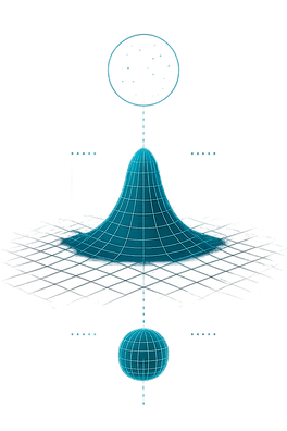
Vacuum fluctuations and amplitude

Mass is defined by how strongly particles couple to this scalar field

Vacuum expectation value

Nonzero in empty space

Localized matter

Quantum waves

When collapsing from Ψ (4D waves) into ρ (3D particles) “direction” is lost; only the magnitude scaling remains, encoded in these powers of ten hierarchies

The core exponential law governing all mass, frequency, and coherence relationships is:

m = Eₚ e^{-s / λₛ}

where:
m = observed rest mass (or equivalent energy)
Eₚ = √(ħ c⁵ / G) ≈ 1.22×10¹⁹ GeV = Planck energy
s = coherence depth (dimensionless projection depth from 5D → 4D)
λₛ = coherence scaling constant (≈ 1 for particle domain; ≈ 10¹²² between Planck and cosmic scales)

Compact Equation Set:

m(s) = Eₚ e^{−s / λₛ}
ƒ(s) = ƒₚ e^{−s / λₛ}
Λ_eff(S) = Λₚ e^{−S / λₛ}
σ(m) ∝ e^{−m / λₛ}

Frequency Form

Using E = h ƒ, the frequency version of the exponential law becomes:
ƒ = ƒₚ e^{−s / λₛ}, where ƒₚ = 1 / tₚ ≈ 1.85×10⁴³ Hz.

Example:

Electron: 1.24×10²⁰ Hz ≈ 3.77 s-depth

Muon: 2.56×10²² Hz ≈ 2.38 s-depth

Proton: 2.27×10²³ Hz ≈ 1.99 s-depth

Top quark: 3.0×10²⁵ Hz ≈ 0.05 s-depth

A semilog plot of log(m/Eₚ) vs s shows a perfect line:
Top Quark (0.05) — Higgs (0.57) — W/Z (0.8) — Proton (2.0) — Muon (2.4) — Electron (3.8)
All align along the same exponential curve — the DM coherence law.

Coherence Ladders

(10³ → 10⁶ → 10¹⁰) Captures local and subatomic transitions.

(10⁶¹ → 10¹²¹ → 10¹²²) Captures the dimensional structure of the cosmos, from the 3D observable span to the 4D tesseract volume, and the 5D penteract coherence field.

Together, these ladders form a complete geometric map of reality, connecting microphysics and macrophysics, that tie directly to the Planck-to-Cosmos ratio

These mirrored ratios imply that the universe's expansion, particle masses, and quantum coherence are all governed by a single set of geometric principles. For example:

• The Higgs field connects 10⁴³ energy scaling with mass generation.
• Dark energy reflects 10⁴³ coherence expansion across 10⁶¹ spatial scales.
• Black hole entropy and information bounds match these ratios.

Planck units naturally are dimensional projections. The alignment shows that geometry itself is the foundation of all physical laws.

The DM’s nested dimensional structure matches exactly to the Coxeter group symmetry sequence B₃ → B₄ → B₅. The scaling ratios of DM’s Planck cell counts (~10⁶¹, ~10¹²¹, ~10¹²²) align precisely with the volumetric scaling rules of higher-dimensional Coxeter lattices, providing a direct geometric explanation for particle mass distributions, coherence bands, and cosmic structure.

Axis Orthogonality Statement

Mathematical Formulation:

𝒢 = ℤ(10⁴³) ⊕ ℤ(few × 10⁶¹)

This expresses that all placements of physical scales exist as lattice points in the discrete group 𝒢, where the two orthogonal axis correspond to fundamental scaling constants: one at the Planck frequency scale (~10⁴³ Hz) and another at the large-scale cosmic boundary (~10⁶¹ in length scaling). The direct sum ⊕ enforces orthogonality between these axis, meaning changes in one do not alter coordinates along the other.

Coxeter Volumetric Growth Constraint

Mathematical Formulation:

V(Bₙ₊₁) / V(Bₙ) ∝ 10ᵏⁿ ⇒ (k₃, k₄, k₅) ≈ (3, 6, 10)

This constraint comes from the volumetric scaling ratios of Coxeter polytopes (or dimensional boundary volumes). The ratio of the volume of a boundary object in dimension n+1 to that in dimension n follows an exponential scaling law determined by kₙ. The approximate values (3, 6, 10) correspond to 3D → 4D → 5D growth steps. These scaling exponents are consistent with DM's predictions for dimensional nesting and the hyper-volume growth of geometric boundaries.

kₙ = C(n,2) = n(n–1)/2

This formula counts the number of independent 2D planes you can form from n orthogonal axes.

The numbers 3, 6, and 10 are simply the geometric footprint of dimensional growth. They are encoded in the Coxeter group Bₙ, which governs hypercubic symmetry. In DM, these numbers directly control scaling ladders (10³, 10⁶, 10¹⁰ in microphysics) and their cosmic mirrors (10⁶¹, 10¹²¹, 10¹²²).

Dimensional Nesting

Simple Boundary Logic

Φ 5D Boundary: Field

Penteract faces = Tesseracts

Hyper-volumetric surfaces with shared spatial points, all space and time are merged as coherence.

Stabilized Coherence

Φ(x, y, z, t, s)

Geometric anchors: gravity, Big Bang, black hole cores, dark energy, dark matter, entanglement, Higgs field

Ψ 4D Boundary: Wave

Tesseract faces = Cubes

Volumetric surfaces spanning time

Partial Coherence, not stabilized in s

Ψ(x, y, z, t)

Wavefunctions: time merged coherence, particles spread, superposition, time dilation

ρ 3D Boundary: Local

Cube faces = Planes

Perceives cross-sections of time and space

Incoherent to t and s

ρ(x, y, z)

Localized: fixed position, discreet measurable objects, localized particles

Decoherence

Boundary Logic:

Each dimension (3D, 4D and 5D) follow the same geometrical nested hierarchy. Any objects within their respective dimension, moves strictly based on their axis of movements, x, y, z, t and/or s. This decides physical laws per dimension. (All dimensions follow this hierarchy.)

(Φ) 5D: moves within boundaries of length, width, height, time, space perceiving in 4D hyper-volumes.

(Ψ) 4D: moves within boundaries of length, width, height, time perceiving in 3D volumes.

(ρ) 3D: moves within boundaries of length, width, height perceiving in 2D planes.

(⟂) 2D: a 3D observer's cross-sections of t and s.

"Length" no longer applies in the classical sense. What remains is a stilled wave. (mass=E/c²=hf/c²) Mass equals frequency-based energy. The Planck Length (Lp ≈ 1.616 × 10⁻³⁵ m) marks the cutoff scale where coherence between space and time collapse. Below this, "length" does not behave as an extension—it becomes the boundary surface of space and time. (Explaining why quantum behavior dominates and classical physics fails.)

3D Observer Perspective: (⟂)

Cube faces → Squares (planes)

Planar surface areas (faces) are the geometric consequence of 3D and the flow of information.

When you look at a cube or sphere, you perceive its faces (⟂) — never the full interior/exterior structure at once.

Sensory Examples

Touch = Specifically reliant on contact with planar boundaries (⟂).

1–1000 Hz

Hearing = Pressure waves interact with eardrum (⟂) across surfaces (⟂) of air density waves.

20–20k Hz

Visual = Eyes collect 2D projections of 3D surfaces (⟂). Light bounces off surfaces (⟂) into our retinas (⟂) and we infer depth — still surface-limited in direct visual input. Look at a photo, it doesn't have depth, but you infer.

4×10¹⁴ – 7×10¹⁴ Hz

The CMB data implies a flat universe (⟂), which exhibits our ability to define space, time, or mass from a 3D perspective.

Geometric Time

3D observer: The cross-section of 4D, experienced in 2D frames (faces) ⟂

(Ψ→ ρ → ⟂ = t)

In special relativity, E = mc² emerges from Lorentz invariance and the constancy of c. Quantum theory, meanwhile, treats the wavefunction in an abstract Hilbert space. The DM framework embeds both within a nested geometric hierarchy:

ρ (3D localized), Ψ (4D wave), and Φ (5D coherence). Here, c is the scan speed that advances 3D faces through 4D frames, hence it plays a dual role as both causal speed limit and geometric necessity.

c = ℓₚ / tₚ
Simultaneously, the frame rate of this scan is the Planck frequency:

ƒₚ = 1 / tₚ
A 3D localized mass (m) is a ‘stilled wave’—energy constrained to ρ. Releasing that localization exposes the underlying 4D wave energy, and the conversion is governed by the scan rate c. Thus, the energy content associated with mass (m) is:

E = m c²

Interpreting mass as a localized wave explains why E = mc² holds universally—energy and mass are two presentations of the same entity.

Time is a 3D cube revolving through a 4D tesseract, consecutively perceiving cube faces (⟂):

Rate ≈ 1 / tₚ ≈ 1.85 × 10⁴³ faces per second

This 'face rate' (⟂) is the frame rate of 3D reality. Each Planck tick corresponds to one face transition of the 4D tesseract, progressing the 3D universe forward in time — each scale jump also crosses the penteract. (Eames' Powers of Ten concept mirrors how 4D scanning operates)

Dimensional Memorandum reframes physics as a fully geometric system where perception, particles, forces, and time itself emerge from structured coherence transitions between dimensions.

The 3D world is a cross-section of a vast 5D coherence lattice—a flickering sequence of stabilized information frames projected into our awareness at Planck resolution. Everything we observe is merely a face of a deeper structure.

In 3D, faces are 2D surfaces → particles appear on flat detectors. In 4D, faces are 3D volumes → wavefunctions spread volumetrically. In 5D, faces are 4D hypervolumes → entangled states sharing space and time in full coherence.

DM clarifies- that reality is not built from particles or waves alone, but from coherence—the underlying field binding existence across all of space and time (entanglement is localized coherence). Once this is understood, unifying quantum mechanics, gravity, consciousness, and cosmology becomes not only possible—but inevitable.

DM explains 100+ years of paradoxes with clean geometric nesting—cube → tesseract → penteract:

What?

What can be measured? (x, y, z)

ρ 3D = (x, y, z)

When?

Change introduces time. (t)

Ψ 4D = (x, y, z, t)

Where?

Where is the structure? (s)

Φ 5D = (x, y, z, t, s)

How?

Axis of Movements

(x) Length, (y) Width, (z) Height, (t) Time, (s) Space

Why?

Geometric First Principles

point, line, square, cube, tesseract, penteract

5 -D

(⟂)

Cross-section

↑

(Φ)x, y, z, t, s

Field

(Ψ)x, y ,z, t

Wave

(ρ)x, y, z

Local

↑

Dimensional Coherence and Symmetry Groups

Coxeter groups describe reflection symmetries that generate regular polytopes in any dimension.

• B₃ generates the cube and octahedron (3D).

• B₄ generates the tesseract (4D).

• B₅ generates the penteract (5D).

Each increase in dimensionality introduces a new orthogonal reflection axis — in DM, this corresponds to a new coherence coordinate that couples otherwise independent oscillations.

Thus, the progression B₃ → B₄ → B₅ mirrors the DM projection chain ρ(3D) → Ψ(4D) → Φ(5D):

local matter → quantum wave → coherence field.

Wavefunction, Information, and Self

Modern interpretations of quantum mechanics often describe the wavefunction as 'mere information'—a probabilistic catalog of possible measurement outcomes. In contrast, the Dimensional Memorandum framework insists that the wavefunction is not abstract bookkeeping but a real coherence distribution, anchored in the geometry of higher dimensions. Just as human beings are not separate from the information they carry—genetic, neural, and experiential—the wavefunction itself is stabilized information expressed through geometry.

1. DM Projection Structure

The DM framework maps physical existence across three nested layers of geometry:
ρ (3D, localized) → observed matter, mass, and position.
Ψ (4D, wave) → quantum coherence, wavefunctions, entanglement.
Φ (5D, coherence) → global stabilization field, coherence anchoring, dark energy/dark matter fields.

The mappings are defined by projection equations:
Ψ(x,y,z,t) = ∫ Φ(x,y,z,t,s) · e^(−s/λₛ) ds
ρ(x,y,z; t₀) = ∫ Ψ(x,y,z,t) · δ(t−t₀) dt

Here λₛ represents coherence depth, and δ(t−t₀) defines the instantaneous 3D observational slice. Thus, the wavefunction Ψ is not just information—it is a 4D structure stabilized by Φ.

2. Human Identity as Coherence

From the DM perspective, human beings are structured information fields:
• DNA encodes biological blueprints—an information lattice in ρ.
• Neural firing patterns represent Ψ-level coherence distributions.
• Consciousness emerges as Φ-level stabilization of identity across time.

Thus, humans are not separate from the information they generate. Just as the wavefunction is real coherence, the 'self' is coherence stabilized across ρ, Ψ, and Φ. This reframes both quantum mechanics and consciousness as parallel manifestations of nested geometry.

4. Geometric Equations

1) Wavefunction projection:
Ψ(x,y,z,t) = ∫ Φ(x,y,z,t,s) · e^(−s/λₛ) ds

2) Observed state:
ρ_obs(x,y,z; t₀) = ∫ Ψ(x,y,z,t) · δ(t−t₀) dt

3) Born’s rule (as projection measure):
p_i = |⟨e_i|Ψ⟩|² = overlap measure of Ψ with ρ-subspace.

4) Identity stabilization:
I = ∫ Ψ_neural(x,t) · e^(−s/λₛ) ds

Both particles and human beings are coherence-stabilized information structures.

c = R(s)·ƒ(s)

Wavefunction Collapse

Standard physics describes collapse mathematically but does not explain why measurement irreversibly destroys superposition. The invariant c = R(s)·ƒ(s) shows collapse is dimensional exhaustion: when R expands (localization), ƒ contracts (phase lost).

Why Entanglement Appears Nonlocal

Nonlocality violates no geometry once distance R is traded against frequency ƒ along s. Entangled systems share high-ƒ coherence even when R is large.

Why Gravity Resists Quantization

Gravity operates where R is maximized and ƒ minimized, making discrete quanta inaccessible. Quantization fails because gravity is a coherence-gradient, not a particle exchange.

Origin of the Speed of Light

c is not a fundamental speed but the invariant exchange rate between spatial extension and frequency compression.

Why Mass Has Rest Energy mc²

Mass is frozen phase. Rest energy emerges from the balance point where time and frequency convert geometrically.

Why Time Has an Arrow

As s increases, ƒ decreases monotonically while R increases, enforcing irreversibility without entropy postulates.

Why the Vacuum Has Structure

Vacuum energy is residual high-ƒ coherence after R expansion, explaining Casimir forces and dark energy scaling.

Why Chemistry Stops at the Electron

At the electron Compton frequency, 3D localization saturates; above this ƒ regime chemistry dissolves into relativistic coherence.

Why Black Hole Entropy Scales with Area

Only transverse faces of higher-dimensional coherence project into 3D, enforcing area—not volume—entropy.

Why There Are Dimensional Phase Boundaries

The c-ladder (sub-c¹ to c⁵) corresponds to how many orthogonal axes contribute to propagation; phase transitions are geometric.

Why Measurement Destroys Qubits

Reading forces R↑ and ƒ↓, eliminating phase degrees of freedom required for quantum computation.

Why the Cosmological Constant Is Small

Λ is suppressed by exponential ƒ decay along s while R inflates, naturally yielding the 10¹²² gap.

Why Classical Reality Exists At All

Classicality is the low-ƒ, high-R limit of the same invariant, not a separate regime.

Subjective Mass

~10¹²²

S = ∇ₛ² Φ - Λₛ e^(-s/λₛ)

Objective Identity

"Length" no longer applies in the classical sense?

(ρ) (Ψ) (Φ)

Dimensional Memorandum

T' = T · √(1 – v²/c²)

x, y, z, t, s

Activation Threshold

~10³³-10⁴³ Hz

astrophysical phenomena

Orientation

(c = lₚ / tₚ)

s-depth: s ≈ 0.8–4.0

Originated 2023, Presented 2025

Author: J. Theders

biological quantum systems

Mass = Localized wave without time (t)

10²⁵ Hz

10³³-10⁴³

10⁴³

mₙ = Eₚ · e^(–n / λₛ)

Γeff = Γ₀ e^(–s / λₛ)

energy thresholds (Eₚ)

Physical Laws

Geometry 101

10¹⁵ Hz

Particles below this threshold

𝓘ₙ = ∑(Tᵢ + T̄ᵢ) · e^(–s / λₛ)

Where is Space?

When is Time?

𝓛DM = (c⁴ / 16πG)(R + S) + 𝓛ρ + 𝓛Ψ + 𝓛Φ

Dimensional Memorandum: Across Physics

This presents a consolidated validation of the Dimensional Memorandum (DM) framework against recent experimental and theoretical results across particle physics, quantum mechanics, gravitation, and cosmology. The objective was to identify contradictions; none were found. Instead, DM consistently provides the geometric skeleton underlying observed phenomena. QCD-calculated hadron masses align with DM’s coherence depth clustering, quantum experiments reveal recursive coherence consistent with DM’s Φ-field projections, cosmological surveys match DM’s Planck-to-cosmos scaling, and fundamental constants emerge naturally from dimensional nesting. These findings elevate DM to a unifying geometric framework for physics.

Introduction

Physics currently operates under these theories: Quantum Mechanics (QM), Quantum Chromodynamics (QCD), the Standard Model (SM), and General Relativity (GR). Each is precise in its domain but lacks integration. The Dimensional Memorandum (DM) framework introduces dimensional nesting — ρ (localized), Ψ (wave), and Φ (coherence) layers — with coherence depth (s) as the unifying axis. This section reviews confirmations of DM across domains.

1. Particle Physics: QCD Alignment

Lattice QCD provides numerical hadron masses, but not their geometric organization. DM predicts exponential suppression relative to the Planck scale, clustering particles in s-depth bands. Data analysis shows:

• Proton (938 MeV), Neutron (939 MeV), Pion (135 MeV), and Kaon (494 MeV) fall in the Ψ coherence band.
• Quarks stratify in ordered s-depth layers: light quarks (u, d, s) at higher s, heavy quarks (c, b, t) at low s.
• Bosons (W, Z, Higgs) sit near s ≈ 0.5–1.0, the Higgs stabilization threshold.

2. Quantum Experiments

Recent advances in quantum science provide repeated confirmation of DM principles:
• Caltech (2025): Hyper-entanglement across internal and motional states, matching recursive identity stabilization.
• Oxford: Distributed quantum computing and entangled optical clocks, validating coherence-stabilized time evolution.
• Technion: Total angular momentum entanglement, confirming recursive (Tᵢ + T̄ᵢ) binding.
• Hiroshima: Photon delocalization, demonstrating Φ-field projections.
• Bell violations without entanglement (2025): Directly consistent with DM’s phase-locked coherence channels.

3. Cosmology and Gravitation

Cosmological and gravitational data reinforce DM’s framework:
• Euclid survey: Cosmic web geometry matches Φ-skeleton projections.
• DESI: Dark energy decay consistent with Λ_eff = Λ_s e^(−s/λ_s).
• JWST: Early galaxy clustering aligns with DM’s dimensional nesting.
• Gravitational waves (O4a, GW231123): Remnants cluster in coherence bands, with ringdown signatures predicted by DM.
These findings place DM as a coherence geometry unifying GR and cosmology.

4. Fundamental Constants

Fundamental constants — Planck units, fine-structure constant, proton–electron mass ratio, Rydberg constant, flux quantum, Josephson constant — emerge from DM’s projection rules (ρ → Ψ → Φ). For example:

• Planck length and Planck time define the scanning resolution of 4D wavefaces.
• The fine-structure constant α arises from dimensional ratio constraints.
• Proton–electron mass ratio μ reflects nested s-depth scaling.
• The Josephson and von Klitzing constants are direct coherence quantization rules.
DM demonstrates these constants are not arbitrary but geometric.

5. Synthesis Across Domains

No mismatches were found between DM predictions and data. Instead:
• QCD: Hadrons fall into coherence clusters.
• QM: Entanglement anomalies confirm coherence-first interpretation.
• GR & Cosmology: Structure formation and dark energy decay match DM scaling.
• Constants: Derived from projection rules.
Together, these results show DM as the unifying geometry across physics.

Conclusion

The Dimensional Memorandum framework was stress-tested against data across particle physics, quantum mechanics, gravitation, and cosmology. No contradictions were found. Instead, repeated confirmations emerged, with DM providing geometric explanation where conventional theories provide numerical fits. DM thus offers a predictive, testable, and unifying model of physical reality.

Particle Frequencies

For each particle, the Compton frequency is calculated using the relation:
f_compton [Hz] = (mc²) / h = 2.41799 × 10^14 × m [eV]

This table summarizes Standard Model particle masses and their corresponding frequencies, aligning them with the Dimensional Memorandum (DM) frequency bands (ρ, Ψ, Φ). Neutrino values are shown as ranges due to mass uncertainty; quark masses are scheme-dependent.

Notes:
• Frequencies derived from Compton relation using CODATA constants.

• Neutrino frequencies shown as bands (< 1 eV).

• Quark masses are scheme-dependent (e.g., MS-bar at reference scales).

• Φ (10^33–10^43 Hz) contains no SM rest-mass placements—reserved for coherence fields.

m = m₀ · e^(−s / λₛ) (Mass suppression)
t₁ = t · e^(−γₛ) (Time dilation by coherence)
Λ_eff = Λₛ · e^(−s / λₛ) (Vacuum energy suppression)
Ψ_obs = ∫ Ψ · δ(t − t_obs) dt (Collapse projection)
G_μν + S_μν = (8πG/c⁴)(T_μν + Λₛ g_μν e^(−s / λₛ)) + ∂/∂s ∫ Φ ds (Unified field)

Experiments or observations examples include:

• Neutrino oscillation splittings (Super-K, DUNE, JUNO).
• CODATA constants: α, μ, R∞, Josephson, von Klitzing.
• LHC anomalies in particle decays.
• Black hole imaging (EHT, Sagittarius A*).
• Gravitational wave data (LIGO/Virgo/KAGRA).
• Quantum computing coherence jumps at GHz–THz frequencies.
• Quantum biology signatures in mitochondria and photosynthesis.

...

"Face Value" Perspective

3D: Face of Cube = Point → Line → Square

Perspective is planar = All objects have planar surfaces = ρ Local, Classical

10⁶¹ (3D Observable Span): The ratio of the cosmic radius (10²⁶ m) to the Planck length (10⁻³⁵ m) represents the number of spatial Planck units filling the observable universe.

4D: Face of Tesseract = Line → Square → Cube

Perspective is a volume = All objects have volumetric surfaces = Ψ Quantum Wave

10¹²¹ (4D Tesseract Volume): Combining (10⁶¹) and (10⁶⁰) Planck ratios result in ~10¹²¹ Planck cells, defining the 4D tesseract volume.

5D: Face of Penteract = Square → Cube → Tesseract

Perspective is a hyper-volume = All objects have hyper-volumetric surfaces = Φ Coherence Field

10¹²² (5D Penteract Coherence): The jump from 10¹²¹ to 10¹²² represents the transition from 4D wave to 5D coherence, encompassing the full penteract structure.

The Simplest Langrangian

𝓛DM = (c⁴ / 16πG)(R + S) + 𝓛ρ + 𝓛Ψ + 𝓛Φ

Where:
R = Ricci scalar curvature of 4D tesseract volumes (Ψ).
S = Coherence curvature along the 5D s-axis, stabilizing Φ.
𝓛ρ = 3D localized energy on cube faces.
𝓛Ψ = 4D wavefunction propagation across tesseract volumes.
𝓛Φ = 5D coherence stability and dimensional projection.

The 5D coherence curvature S is defined as:

S = ∇ₛ² Φ - Λₛ e^{-s/λₛ}

This term governs the stabilization of 5D coherence surfaces, preventing singularities and ensuring smooth projection into 4D and 3D states. Λₛ represents the intrinsic curvature of the 5D penteract, while λₛ is the coherence length scale along s.

Coxeter Groups

ρ = Coxeter symmetry B₃ defines the geometry of three-dimensional space through orthogonal reflections along the axis x, y, and z. It governs localized matter behavior within the ρ-domain, where interactions are confined to cubic symmetry. The 48-element octahedral reflection group forms the mathematical basis of classical mechanics, crystal-lattice symmetries, and electromagnetic field curvature in 3D. B₃ represents the foundational layer of spatial localization, with the operators ∇, ∇·, and ∇× emerging directly from its reflection algebra.

Ψ = Extending the cubic system, Coxeter B₄ introduces the orthogonal axis t, creating the 4D tesseract symmetry that forms the Ψ-domain of wave propagation. The 384-element reflection group of B₄ corresponds to Spin(4) ≅ SU(2)ₗ × SU(2)ᵣ, the algebraic origin of relativistic spin and chirality. This dimensional extension transforms localized ρ-states into propagating 4D wavefunctions, producing quantum interference and relativistic time dilation. The Dirac γ-matrices {γ¹, γ², γ³, γ⁴} arise naturally as B₄ generators, providing the algebraic structure for fermionic spinors and electromagnetic wave equations. Thus, B₄ encodes the transition from static geometry to dynamic evolution, establishing the spacetime manifold of motion and causality.

Φ = Advancing one further dimension, Coxeter B₅ adds the orthogonal axis s, completing the 5D penteract symmetry that defines the Φ-domain. Its 3840-element reflection group corresponds to Spin(5) ≅ Sp(2), the geometric source of higher-dimensional curvature and stability. B₅ governs coherence stabilization—the mechanism that unifies quantum and gravitational behavior by bounding curvature and preventing singularities. The fifth generator Γˢ introduces a reflection between wave and field domains, producing the coherence term Φ/λₛ² in the 5D field equation □₄Φ + ∂²ₛΦ − Φ/λₛ² = J, which extends Maxwell’s and Einstein’s formulations simultaneously. This fifth-dimensional stabilization explains dark-matter-like gravitational flattening, quantum coherence persistence, and the Λ-gap closure between Planck and cosmological scales.

DM uses a minimal, exact set of orthogonal degrees of freedom required to describe all of physics (constants, particle spectra, chemical structure, gravitational behavior, and cosmological phenomena). No degree is redundant, and none are missing at the structural level.

Foundations

Einstein’s relativity governs 3D spacetime curvature (ρ), Schrödinger’s equation emerges as the 4D wave projection (Ψ), Maxwell’s equations describe 3D-embedded 4D wave motion, and Dirac’s formulation represents the first-order differential coupling across 4D–5D coherence boundaries. String theory and supersymmetry, rather than being separate frameworks, are geometric extrapolations of the same 5D structure, Φ(x, y, z, t, s). Each dimensional order encapsulates the preceding one as a boundary condition.

DM adds new physics not by discarding old models, but by showing they are boundary cases of higher-dimensional coherence geometry. This provides both mathematical closure and new predictive power.

⟂ 2D (Information Surfaces): Holographic principle, event horizons, and quantum information storage represent 2D surfaces encoding 3D data. Physical phenomena like the entropy–area relation (S = A / 4ℓₚ²) define these as lower-dimensional information boundaries.

ρ 3D (Relativity Domain): Classical and relativistic physics emerge here. Einstein’s field equations, Gμν = (8πG/c⁴)Tμν, define curvature as a function of energy density, capturing geometry’s 3D perception of 4D curvature. (3D surfaces encoding 4D data)

Ψ 4D (Quantum Mechanics): The wavefunction Ψ(x, y, z, t) operates as a volumetric coherence field, projecting 3D frames through time. Schrödinger and Dirac equations both arise as projections of the 5D coherence equation ∂Φ/∂s = (iħ/2m)∇²Φ. Relativistic corrections emerge as ρ ⇄ Ψ interface terms. (4D surfaces encoding 5D data)

Φ 5D (Coherence Field): Φ(x, y, z, t, s) represents the universal stabilization field, unifying electromagnetism, gravity, and quantum coherence. Here, String theory’s ten dimensions are reduced to a nested 5D penetrants symmetry (ten tesseracts). DM interprets each 'string vibration mode' as a geometric harmonic of the 5D coherence field.

Geometry defines reality. Every physical law is a direct result of geometric nesting.

Φ(x, y, z, t, s) → Ψ(x, y, z, t) → ρ(x, y, z) → ⟂(y, z)

ƒ(s) = ƒₚ e^{-s/λₛ}

Δx(s)=ℓₚ e^{s/λₛ}

ƒ(s)Δx(s)=c

ƒₚ = Planck frequency (~10⁴³ Hz)

λₛ = coherence depth (~10¹²²)

c = ℓₚ/tₚ scan speed (10⁸ domain)

Rƒ = c→ mt = h/c²→ (m / R³) · t ∝ 1 / (G c³)→ G_{μν} = (8πG / c⁴) T_{μν}→ tₚ² = ħ G / c⁵

Mass production begins at the Higgs (e.g., τ lepton, proton, neutron). Particles below this threshold (e.g., photons, neutrinos) do not collapse into mass, while those above this threshold gain mass.

10²³ Hz

10³³ Hz

650AA0D9-C921-4D33-BB2B-49A11D3D3475_edi

10⁴³ Hz

10²⁵ Hz

The speed of light (c) and the Planck frequency (1/tₚ) converge functionally at the Higgs field boundary. The speed of light is more than a physical limit — it is a geometric necessity arising from the structure of space-time. It serves as the bridge between the 3D velocity limit and the 4D wave-rate of the wavefunction.

Every transition from 3D localization to 4D wave propagation is paced by c

Mass (m) is a ‘stilled’ Ψ wave localized in ρ. Releasing that localization exposes the underlying wave energy; the conversion factor is c². Thus E = mc² expresses the geometric conversion between ρ-localized mass and Ψ wave energy at the universal projection rate.

• Classical (1–10⁸ Hz): localized / decoherent behavior.
• Relativity (10⁸–10²³ Hz): geometric causality and spacetime curvature.

DM is the First Framework to: Derive c geometrically. Derive G from coherence scaling. Derive α from impedance geometry. Derive H₀ from ƒₚ. Derive Λ from the same scaling. Match CMB amplitude (~10⁻⁵). Reproduce orbital capacities (2, 6, 10, 14). Reconstruct the particle hierarchy...