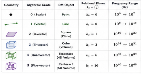
Dimensional Memorandum
.png)
A hub for scientific resources.

The Dimensional Memorandum Framework (DM)
We restore simplicity by showing that all scales, from quantum to cosmic, are governed by the same geometry.
Explaining why multiple "unrelated" anomalies share the same root.
Note:
Nothing in this work is intended to discredit the remarkable achievements of modern physics. Quantum Mechanics, Quantum Field Theory, and General Relativity remain among the most successful theories ever constructed. Their predictive power, internal consistency, and empirical adequacy are not in question. Instead, we clarify the explanation that underlies these theories.
The Dimensional Memorandum (DM) framework preserves the Standard Model (SM), General Relativity (GR), CODATA-defined constants, and high-energy collider measurements. DM reproduces all established physical equations exactly within current experimental precision. Schrödinger, Klein–Gordon, Dirac, Maxwell, and Einstein equations remain unchanged.
The real challenge is shifting perspective from fragmented models to unified structure.
At its deepest level, physics is not simply a collection of equations, but an attempt to answer a single foundational question:
What is the Underlying Structure of Reality that Gives Rise to All Observed Physical Laws?

This includes explaining:
• Why spacetime exists
• Why quantum mechanics governs probabilities
• Why gravity curves spacetime
• Why particles and forces have their specific structure
• Why physical constants have fixed values
• Why information and entropy play a fundamental role
Hypothesis: A physical system is described by an algebraic set of laws (L), including dynamical equations, scaling relations, symmetry generators, entropy relations, and open-system evolution equations. If these laws are internally consistent and structurally convergent, then there exists an underlying geometric structure (G) such that:
L = A(G)
where A denotes the algebraic representation of G.
The recovery of the geometric structure whose constraints produce the observed algebraic laws:
G = A⁻¹(L)
Meaning:
Algebra defines the allowed dynamics of a structure.
Geometry, at its most fundamental sense, is the mathematical description of structure.
By analyzing physical equations collectively, one can reconstruct the geometry they are describing.
Foundational Patterns
Recognizing Shared Structure
When measurements are expressed in their most reduced form, they consistently map onto:
Orthogonal directions • Relational planes • Boundary constraints • Scaling invariants
The central finding is that all physical systems evolve continuously along a set of orthogonal axes:
𝓖 = (∇, ∂ₜ, ∂ₛ)
where ∇ describes spatial structure, ∂ₜ describes temporal evolution, and ∂ₛ describes evolution along the coherence axis.
Gradient scaling:
𝒪(s) ∼ Lᴰ⁽ˢ⁾, 2 ≤ D(s) ≤ 3
Dimensional behavior evolves smoothly.
Discrete resonances:
sₙ = (n + α)λₛ
Observable structures arise as resonance-stabilized states.
Any object existing within a given dimension must structurally possess all such axes:
Mⁿ = {x¹, x², ..., xⁿ}
Then any physical object O ⊂ Mⁿ satisfies:
O = O(x¹, x², ..., xⁿ}
An object embedded in an n-dimensional manifold necessarily possesses n independent degrees of freedom.
We identify axes, relational capacity, boundary constraints, and symmetry as the fundamental primitives.
First Primitive: Axis of Movement
An axis of movement is an independent generator along which a state can vary. Vectors are weighted movements along axes; bivectors are coupled two-axis movements; tensors are multi-axis relation containers; tensor networks are organized axis-index relations; and observable physics is the boundary-projected output of this relational architecture. This primitive unifies Coxeter-Clifford structure, tensor-network geometry, scale-flow laws, and gravity-emergence into one clean starting point.
Before a vector has components, before a field changes, before a particle moves, there must be an allowed direction of change.
Axis of Movement is an independent generator of possible state change. A state can be displaced, updated, phased, transported, projected, or transformed along that axis. The axis is primitive because it defines a possible movement before any specific object moves along it.
1. Independent axis define possible directions of variation;
2. Vector and tensor products define relations among those directions;
3. Fields distribute those relations over a manifold;
4. Differential laws determine their evolution;
5. The frequency ladder specifies the rate and scale at which a state varies.
1. Allowed Motions and Interactions Within a System are Strictly Constrained by the Dimensional Structure in Which It Exists.
Changing the axis changes the accessible information, and therefore the observed physics.
Axis extension corresponds to increasing dimensionality, while axis reduction corresponds to projection. These operations determine changes in dynamics, relational capacity, and algebraic structure.
A system defined on an n-dimensional manifold Mⁿ with coordinates xᴬ extends to Mⁿ⁺¹ by introducing a new independent coordinate:
Mⁿ → Mⁿ⁺¹, (xᴬ) → (xᴬ, xⁿ⁺¹)
The derivative operator becomes:
∇ₙ = eᴬ ∂_A
∇ₙ₊₁ = ∇ₙ + eⁿ⁺¹ ∂ₙ₊₁
Adding an axis introduces a new independent direction of motion and differentiation.

Extending to spacetime introduces time derivatives:
∇ = (∂_x, ∂_y, ∂_z)
∇² = ∂_x² + ∂_y² + ∂_z²
The Schrödinger equation:
iħ ∂ₜΨ = −(ħ²/2m) ∇²Ψ + VΨ
□ + m²c²/ħ²)Ψ = 0
Coupling between time and spatial derivatives generates wave behavior, phase evolution, and interference.
A relativistic wave:
∂_μ = (1/c ∂ₜ, ∇)
□ = (1/c²) ∂ₜ² − ∇²
This combines space and time symmetrically under spacetime geometry.
axis:
Ψ(x,y,z,t) → ρ(x,y,z)
ρ(x,y,z) = |Ψ(x,y,z,t)|²
Extending further introduces an additional derivative:
∂_M = (∂ₛ, 1/c ∂ₜ, ∇)
□₅ = (1/c²) ∂ₜ² − ∇² − ∂ₛ²
Observable states arise through projection along the additional axis:
Ψ = ∫ Φ e^(−s/λₛ) ds
axis:
Φ(x,y,z,t,s) → Ψ(x,y,z,t) → ρ(x,y,z)
Ψ(x,y,z,t) = ∫ Φ(x,y,z,t,s) e^(−s/λₛ) ds
The number of accessible axes determines the full range of admissible dynamics.
Adding an axis increases degrees of freedom, expands relational structure, and enlarges the space of admissible dynamics.
Conversely, reducing accessible degrees of freedom yields effective descriptions of the underlying system.
The gradient changes through dimensional extension produce the full range of observed physical behavior.

1.1 Axis of Movement → Algebraic Generator
eᵢ eⱼ + eⱼ eᵢ = 2 gᵢⱼ
Each independent axis of movement corresponds to a Clifford basis vector eᵢ. These generators define the geometric algebra of the system, encoding directions of motion and allowable transformations.
1.2 Relational Capacity and Plane Structure
kₙ = n(n-1)/2
dim Clₙ = 2ⁿ
The number of independent bivector planes corresponds to relational capacity kₙ. These quantities grow systematically with each added axis.
3 axes Cl₃: Spatial ∇ (M³)
Cl₃: {e₁, e₂, e₃}, dim = 8, k₃ = 3
This describes three-dimensional space. Its bivectors correspond to spatial planes, governing rotations and localized particle structure. This level corresponds to the ρ-layer of matter and boundary geometry.
4 axes Cl₄: Spacetime ∂ₜ (M⁴)
Cl₄: {e₁, e₂, e₃, e₄}, dim = 16, k₄ = 6
F = (1/2) F_{μν} γ^μ ∧ γ^ν
Adding the time axis produces Cl₄. The six bivectors correspond to spacetime planes, including those underlying the electromagnetic field tensor. This level corresponds to the Ψ-layer of wavefunctions and relativistic dynamics.
5 axes Cl₅: Coherence ∂ₛ (M⁵)
Cl₅: {e₁, e₂, e₃, e₄, e₅}, dim = 32, k₅ = 10
Adding the coherence axis s produces Cl₅. The additional bivectors introduce new planes involving coherence, enabling entanglement structure, projection dynamics, and stabilization effects. This corresponds to the Φ-layer.
Φ(x,t,s) → Ψ(x,t) → ρ(x,t)
Ψ = ∫ Φ e^{-s/λₛ} ds
The higher-dimensional Clifford structure projects down through successive layers. Cl₅ encodes the full coherence structure, Cl₄ encodes wave evolution, and Cl₃ encodes observable matter.
Rotations in Clifford algebra are generated by bivectors. Thus, spin and orbital structure arise naturally from plane geometry. As the algebra extends, the space of possible rotational and coherence transformations expands. Each step increases dimensionality, relational capacity, and physical richness.

2. The Vector Structure and Axis Structure Align Directly with Relational Capacity as:
kₙ = n(n−1)/2, Under Axis Extension: kₙ₊₁ = kₙ + n
This quantity corresponds to the number of independent bivector planes, antisymmetric tensor components, and generators of the rotation group SO(n). It defines the maximum possible relational structure.
Quantum stability = maximize s and kₙ with environmental coupling minimized.
eᵢ → eᵢ ∧ eⱼ → Clₙ → Pin(n), Spin(n) → W → Nₙ → ∂M → Ψ → τ_c → Q
Example:
k₃ = 3 → k₄ = 6 (+3)
k₄ = 6 → k₅ = 10 (+4)
Clifford algebra:
dim(Clₙ) = 2ⁿ
Under axis extension:
dim(Clₙ₊₁) = 2 dim(Clₙ)
The metric tensor extends as:
g_AB → [g_{μν} 0]
[0 gₛₛ]
Leading to the generalized line element:
ds² = g_{μν} dx^μ dx^ν + ε ds²

M²
Axes: (x,y)
k₂ = 1
Pairs: (xy)
M³
Axes: (x,y,z)
k₃ = 3
Pairs: (xy), (xz), (yz)
Grade:
n = 3: 1+3+3+1 (8)
Symmetry operations:
|B₃| = 48
M⁴
Axes: (x,y,z,t)
k₄ = 6
Pairs: (xy), (xz), (xt), (yz), (yt), (zt)
Grade:
n = 4: 1+4+6+4+1 (16)
Symmetry operations:
|B₄| = 384
M⁵
Axes: (x,y,z,t,s)
k₅ = 10
Pairs: (xy), (xz), (xt), (xs), (yz), (yt), (ys), (zt), (zs), (ts)
Grade:
n = 5: 1+5+10+10+5+1 (32)
Symmetry operations:
|B₅| = 3840
Each step adds new pairwise relations between the new axis and all previous axes.
2.1 Amplitude Normalization
ψⁿ = (1/√kₙ) Σ ψₐ
|ψ|² distributes as 1/kₙ per channel
2.2 Action Scaling
Sⁿ = Σ gₙ Sₐ
gₙ ~ 1/kₙ (fixed total action)
2.3 Information Functional
λ kₙ wₙ = ħ²/(8m)
wₙ = ħ²/(8m λ kₙ)
2.4 Coupling Scaling
gₙ ~ g₀/kₙ (fixed sum)
gₙ ~ g₀/√kₙ (fixed norm)
2.5 Interference
|ψ|² = (1/kₙ) Σ |Aᵢⱼ|² + (1/kₙ) Σ Aᵢⱼ Aₖₗ cos(Δθ)
2.6 Entanglement
E ∝ N_cross / kₙ
Cross-channel connectivity.
2.7 Bell Violation
|S| ≤ 2 (classical), |S| ≤ 2√2 (quantum)
Arises from non-factorizable coherence.
2.8 Wavefunction
ψ = (1/√kₙ) Σ Aᵢⱼ e^{iθᵢⱼ}
Normalized over relational channels.
2.9 Density Matrix
ρ = (1/kₙ) Σ Aᵢⱼ Aₖₗ e^{i(θᵢⱼ−θₖₗ)} |ij⟩⟨kl|
2.10 Decoherence
ρᵢⱼ,ₖₗ → 0
S_CHSH(t) ≈ 2√2 e^(−Γt)
2.11 Entropy
S = −k_B Σ p ln p
Entropy from projection information loss.
2.12 Electromagnetic Structure
Measured electric and magnetic fields combine into F_{μν}
with independent components:
k₄ = 4(4−1)/2 = 6

3 axes = 1 + 3 + 3 + 1
4 axes = 1 + 4 + 6 + 4 + 1
5 axes = 1 + 5 + 10 + 10 + 5 + 1
Clifford algebra begins with vectors and a metric:
uv + vu = 2g(u,v)
An orthonormal Euclidean basis, eᵢ² = 1 and eᵢ eⱼ = - eⱼ eᵢ for i ≠ j. The product of two vectors decomposes into a symmetric inner product and an antisymmetric exterior product:
uv = u · v + u ∧ v
The wedge term u ∧ v is an oriented plane. In DM this is the first relational object. The number of independent planes is the dimension of the bivector sector:
kₙ = dim Λ²(V) = C(n,2) = n(n−1)/2
Relational capacity in an n-dimensional sector.
The same number is the dimension of so(n), the Lie algebra of rotations. This is not accidental: rotations occur in planes. A bivector is therefore both an oriented plane and an infinitesimal generator of rotation.
The full Clifford algebra decomposes by grade:
Clₙ = Λ⁰ ⊕ Λ¹ ⊕ Λ² ⊕ ··· ⊕ Λⁿ, dim Λʳ = C(n,r), dim Clₙ = 2ⁿ
Relational capacity kₙ counts independent oriented 2-plane relations in an n-dimensional manifold. Tensor networks generalize this idea into graph-based relational capacity. The capacity is not only determined by the ambient dimension; it is also determined by the active network edges and their bond dimensions.
Manifold relational capacity:
kₙ = n(n-1)/2 = dim Λ²(Mⁿ)
Tensor-network relational capacity proxy:
K_TN = Σ_{edges e} log(χ_e)
If all bonds have χ:
K_TN = |E_graph| log(χ)
kₙ describes the relational plane capacity of a geometric sector; K_TN describes the information-channel capacity of a tensor network embedded in or representing that sector.
A tensor network naturally distinguishes between internal and external structure. External legs are the boundary indices, corresponding to physical degrees of freedom. Internal bonds are hidden relational structure. After contraction, the internal structure is not directly observed; it supports the boundary state.
In standard quantum mechanics, the state of many subsystems is represented by a high-rank tensor of amplitudes. Tensor networks factor that tensor into smaller local tensors connected by internal bond indices. These bonds encode entanglement and define an information geometry. This is a concrete mathematical bridge between relations, boundaries, coherence, and observable physics. The result is a disciplined placement of tensor networks inside the DM chain: occupied relational structure becomes a boundary wavefunction through projection and contraction.
Quantum mechanics stores physical information in amplitudes of a state vector or wavefunction.
For many-body systems, the amplitude object becomes exponentially large: dᴺ coefficients for N subsystems of local dimension d.
Tensor networks compress this object by factorizing it into local tensors connected by bond indices.
Bond indices encode entanglement channels; bond dimension chi controls how much relational information can pass through a cut.
The network graph is not decoration: it is the geometry of quantum information used to represent the state.
In DM, tensor networks occupy the Nₙ → partial M → Ψ segment of the chain, turning hidden relational structure into boundary-observable wavefunction data.
eᵢ → eᵢ ∧ eⱼ → kₙ → Nₙ → ∂M -> Ψ → τ_c → Q
Local tensors + bonds → network geometry → boundary legs → contracted wavefunction Ψ
For a composite quantum system, the state is not merely a list of particles. It is a structured amplitude object over all allowed joint configurations. If the system has N subsystems, each with local dimension d, a general state requires d^N complex amplitudes. This exponential growth is the computational challenge that tensor networks address.
|Ψ⟩ = Σ_{i₁,i₂,...,i_N} Ψ_{i₁ i₂ ... i_N} |i₁ i₂ ... i_N⟩
Number of amplitudes for N local systems: dᴺ
The coefficient array Ψ_{i₁...i_N} is a high-rank tensor. The wavefunction is therefore already a tensorial object. Tensor networks do not add tensor structure from outside; they expose a useful factorization of a tensor structure already present in quantum mechanics.
Tensor Networks Factor the Wavefunction
A tensor network rewrites one large amplitude tensor as a contraction of many smaller tensors. The external indices correspond to physical degrees of freedom. The internal indices are summed over and represent hidden relational channels between parts of the system.
Ψ_{i₁ i₂ ... i_N} = Σ_{α₁,...,α_{N-1}} A^{i₁}_{α₁} A^{i₂}_{α₁α₂} ... A^{i_N}_{α_{N-1}}
Capability Functional
Q = k_eff N_n τ_c R (1 - p_L)
This mapping is not a standard tensor-network theorem; it is a DM engineering functional that organizes the measurable ingredients of useful quantum structure. For tensor-network quantum mechanics, the terms can be interpreted as follows:
k_eff: active network connectivity / active geometric planes → How many relational channels actually participate
Nₙ: occupied tensor-bond structure → How much of the possible network structure is used
τ_c: coherence lifetime of represented state → How long quantum phase/entanglement remains useful
R: redundancy, code distance, ensemble support, tensor encoding → How much protection or repetition preserves information
p_L: logical error or truncation/loss probability → Probability that useful relational information is lost

3. Observable Information is Boundary-Limited:
∂Mᴰ = Mᴰ⁻¹
Each level of physical description is a reduced representation of a higher-dimensional structure. Information propagates in physical systems as a sequence of boundary-to-boundary projections across dimensions. Observable physics arises from this recursive encoding process. Accessible information = ∂Mᴰ⁻¹
M⁵ (field) → M⁴ (wave) → M³ (local) → M² (boundary measure)
Information scaling: Iₙ ∼ (Vₙ₋₁ / ℓₚⁿ⁻¹) · (1 / tₚ)
AdS/CFT is a formal realization of this principle. The DM framework adopts the same boundary-encoding logic, but extends it by incorporating axis-dependent accessibility, coherence projection, and a direct link to observable quantum and classical regimes.
DM makes the projection axis explicit. Spatial, temporal, and coherence projections do not reveal the same subset of boundary information. The bulk-to-boundary map of AdS/CFT and the projection structure of DM are mathematically aligned at the level of kernel-based reconstruction.
Holography is one instance of a broader boundary-projection principle.

(Φ) ∂M⁵ = M⁴: Information encoded in M⁴ hypervolumes (coherence) → (∂ₛ)
The 5 axes → 4 axes projection yields the field → wave: ψ(x,t) = ∫ ds Φ(x,t,s) e^(−s/λₛ)
(Ψ) ∂M⁴ = M³: Information encoded in M³ volumes → (∂ₜ)
The 4 axes → 3 axes projection yields observable probability density: ρ(x,t) = |ψ(x,t)|²
(ρ) ∂M³ = M²: Information encoded in M² areas (localized observation) → (∇)
The 3 axes → 2 axes projection yields area-encoded information: S ∼ k_eff |∂A|
3.1 Observable Structure
ρ(x,y,z) = |Ψ(x,y,z,t)|² lies on M⁴
with ∂M⁴ = M³
3.2 Human Perception
Receive 2D projections and reconstructs 3D reality
∂M³ = M² → reconstructs M³
3.3 Boundary Density
|Ψ|² represents density on the boundary.
Measurement accesses only boundary-compatible structure.
3.4 Gravity
S = ∫ √(-g)R + ∫ √|h|K
Boundary geometry encodes gravity.
3.5 Information and Boundary Scaling
Black hole thermodynamics gives:
S ∼ A / ℓₚ²
Information scales with boundary area
3.6 Casimir Effect
Two conducting plates restrict vacuum electromagnetic modes. This boundary restriction produces a measurable force, demonstrating that vacuum fluctuations are boundary-dependent.
3.7 Quantum Hall Effect
Conducting states exist at system boundaries rather than in the bulk. Transport occurs through edge channels.
3.8 Topological Insulators
Surface states exist even when the bulk is insulating. These states are protected by boundary topology and are directly observable.
3.9 Cavity Modes
In resonant cavities, boundary geometry determines allowed standing-wave modes. Node and antinode structure is completely defined by boundary conditions.
Boundary conditions determine the allowed solutions.
Reality is a multi-axis structure, and observation corresponds to projection of higher-dimensional geometry onto lower- dimensional boundaries as it evolves.
4. A Cross-Section is the Intersection of a Higher-Dimensional Manifold:
Mᴰ ∩ Σᴰ⁻¹
Each observable slice in the cascade M⁵ → M⁴ → M³ → M² is not merely a lower-dimensional restriction, but a symmetry-conditioned cross-section whose accessible structure is counted by relational capacity kₙ organized by Coxeter symmetry |Bₙ|, and realized through plane-harmonic mode capacity Nₙ (48 / 384 / 3840 hierarchy).
The accessible content is filtered by the symmetry and relational structure of the slice: Mₙ₋₁ = Sliceₐ(Mⁿ)
Cross-sections are both geometric and informational: they reduce dimension and simultaneously select which boundary-encoded information remains accessible. The number kₙ counts the independent planes, bivectors, or relational channels in n dimensions. These planes are the fundamental slots in which harmonics, rotations, and interaction channels are organized. While Bₙ count the reflection, sign-flip, and permutation operations of the n-dimensional sector. They therefore measure the total discrete symmetry closure of each slice.
Plane-harmonic mode capacity
Nₙ = kₙ × 2 × 2 × 4
A local plane-harmonic basis is built from: (1) plane count kₙ, (2) two quadratures, (3) two propagation directions, and (4) four minimal sign/orientation sectors. For the 3D local slice this gives:
N₃ = 3 × 2 × 2 × 4 = 48
The local 3D plane-harmonic basis closes exactly on the Coxeter count |B₃| = 48.
(M⁴) 4 axis cross-sections and the 384 structure
k₄ = 6
|B₄| = 384
The 4D slice introduces six independent spacetime planes. These support the bivector structure of the electromagnetic field and the spin-generating structure of relativistic field theory. The 384 count is the symmetry-complete reorganization capacity of this 4D interface layer.
F_{μν} ⇄ Λ²(R⁴), dim Λ²(R⁴) = 6
The 4D slice is the natural cross-section in which wavefunction and field structure appear.
(M⁵) 5 axis cross-sections and the 3840 structure
k₅ = 10
|B₅| = 3840
The 5D layer is the coherence bulk. It contains the full ten-plane relational structure. This is the maximal structural support for coherence, entanglement, and higher-dimensional stabilization.
Φ(x,y,z,t,s)
The 5D coherence field is therefore the hypervolume whose lower-dimensional slices generate all observable physics.
4.1 Higher-Dimensional Extension (4D → 3D)
Ψ(x,y,z,t) ∈ M⁴ → Ψ_obs = M⁴ ∩ Σ³.
4.2 Measurement
ψ_obs = Mᴰ ∩ Σᴰ⁻¹
P = |ψ_obs|² / ∫ |ψ_obs|²
Measurement = boundary slice selection.
4.3 Time
M⁴ = ⋃ Σₜ³
Time = ordering of slices.
Entanglement:
Φ_AB ≠ Φ_A Φ_B ⇒ ψ_AB ≠ ψ_A ψ_B
ƒ ≈ 10⁻¹⁸ Hz (time)
S ≈ 10¹²² (capacity)
4.4 Born Rule is Cross-Section Density
ρ(x,y,z) = |Ψ(x,y,z,t)|²
4.5 Relational Capacity Reduction
k₅ = 10 → k₄ = 6 → k₃ = 3
Decoherence = restriction of cross-sections.
ρᵢⱼ(t) = ρᵢⱼ(0) e^(−Γ t)
Γ(s) = (α₀/kₙ) e^(−β s/λₛ)
Γ ≈ 10⁻¹²² → 10⁻⁶¹
k₅ = 10 → k₃ = 3
Interference = overlapping cross-sections.
5. All Physical Quantities Organize into Dual Exponential Sectors Along a Single Coherence Coordinate (s), with Invariant Conjugate Products:
Expanding Sector: R, t, N, A, S grow with s.
Contracting Sector: ƒ, E, m, ρ_Λ, Γ decay with s.
Logarithmic coordinate s, termed coherence depth, represents the projection depth from a higher-dimensional coherence field into observable spacetime. This coordinate is defined by:
s = λₛ ln(R / ℓₚ),
Establishing an exponential correspondence between scale, frequency, and energy. Along this axis, fundamental quantities separate into two conjugate sectors.
Expanding:
R(s), t(s), N(s), A(s), S(s) ∝ e^{+s/λₛ}
R(s) = ℓₚ e^{s/λₛ}
t(s) = tₚ e^{s/λₛ}
N(s) ~ e^{s/λₛ}
A(s) ~ ℓₚ^2 e^{2s/λₛ}
S(s) ~ e^{2s/λₛ}
Contracting:
ƒ(s), E(s), m(s), T(s), ρ_Λ(s), Γ(s) ∝ e^{-s/λₛ}
ƒ(s) = ƒₚ e^{-s/λₛ}
E(s) = Eₚ e^{-s/λₛ}
m(s) = mₚ e^{-s/λₛ}
T(s) = Tₚ e^{-s/λₛ}
ρ_Λ(s) ~ ρₚ e^{-2s/λₛ}
Γ(s) ~ (α₀/kₙ) e^{-β s/λₛ}
Invariant products preserved:
R(s) ƒ(s) = c
t(s) ƒ(s) = 1
E(s) t(s) = h
m(s) t(s) = ħ / c²
R(s) m(s) = ℓₚ mₚ
k_B T(s) t(s) = h
Expansion along s maintains fundamental physical constants while redistributing scale, energy, and information.
Linear quantities scale as e^(s/λₛ)
Boundary quantities scale as e^(2s/λₛ)
Gravity:
G ρ(s) t(s)² / c² = e^(−2s/λₛ)
curvature of boundary entropy
Boundary / Entropy:
A(s) ∝ e^(2s/λₛ), S(s) ∝ e^(2s/λₛ)
Boundary quantities scale quadratically:
A ∝ R² → e^(2s/λₛ)
e²⁸⁰ ≈ 10¹²²
Vacuum energy:
ρ(s) ∝ e^(−2s/λₛ)
ρ ≈ 10⁻¹²²
Ratio Between the Planck Frequency and the Hubble Expansion Rate Defines a Fundamental Scale:
ƒₚ = 1 / tₚ ≈ 1.85 × 10⁴³ Hz
H_0 ≈ 2.2 × 10⁻¹⁸ s⁻¹
ƒₚ / H₀ ≈ 10⁶¹
The square of this ratio yields:
(ƒₚ / H₀)² ≈ 10¹²²
Scale of the observable Ladder
Planck scale:
ƒₚ ≈ 10⁴³ Hz
ℓₚ ≈ 10⁻³⁵ m
Cosmic scale:
ƒ ≈ 10⁻¹⁸ Hz
R ≈ 10²⁶ m
Length span:
10⁻³⁵ → 10²⁶ = 61
Frequency span:
10⁴³ → 10⁻¹⁸ = 61
Midpoint (half exponent)
Length midpoint:
ℓ(mid) ≈ 10^{-4.5} m ≈ 3 × 10⁻⁵ m
Frequency midpoint:
ƒ(mid) ≈ 10^{12.5} Hz ≈ 3 × 10¹² Hz
Using:
R(s) = ℓₚ e^{s/λₛ}
Depth:
s/λₛ ≈ 140
Midpoint:
s/λₛ ≈ 70
The midpoint corresponds to the terahertz regime and mesoscopic length scales.

Frequency
Domain
Physical Interpretation
IR Boundary
10⁻¹⁸ Hz
Boundary
Cosmological limit
Classical Threshold
10⁰ Hz
Edge
Macroscopic emergence
(s/λₛ ≈ 70)
10^12.5 Hz
Interior
Balanced mesoscopic regime
Field Threshold
10²⁵ Hz
Edge
High-energy structure
UV Boundary
10⁴³ Hz
Boundary
Planck limit
Observable physical reality is confined to the interior band of the coherence ladder, while the ultraviolet and infrared endpoints define the limits of projection.
E = h ƒ and ƒₚ = Eₚ/h, or E = ℏ ω and ω_P = 1/tₚ.
The Compton relation locks mass, frequency, and length into one scaling structure. Energy-frequency and mass-energy relations:
E = h ƒ
E = m c²
Equating the two gives:
m = (h/c²) ƒ
The Compton wavelength is:
λ𝒸 = h/(m c)
Substituting m = h ƒ/c² gives:
λ𝒸 = h / [ (h ƒ/c²)c ] = c/ƒ

6. The ×10 Scaling Ladder From 10⁰ to 10⁴³:
10ⁿ → 10ⁿ⁺¹ = 10 × 10ⁿ
The ×10 ladder defines a unified axis of physical reality. Increasing frequency corresponds to increasing energy density and mass, while compressing space and time. Curvature rises quadratically with scale compression.
If frequency ƒ = log10, then:
Energy: E = h ƒ → increases
Time: t = 1/ƒ → decreases
Length: λ = c/ƒ → decreases
Mass: m = E/c² = (h/c²) ƒ → increases
Momentum: p = E/c = (h/c) ƒ
10⁴³ represents 43 sequential multiplications by 10: 10⁴³ = 10 × 10 × 10 × ... (43 times)
10⁰ = 1
10¹ = 10
10² = 100
10³ = 1000
10⁴ = 10000
etc.
6.1 These values define the coherence origin (s = 0):
Planck length: ℓₚ = 1.616 × 10⁻³⁵ m
Planck time: tₚ = 5.391 × 10⁻⁴⁴ s
Planck mass: mₚ = 2.176 × 10⁻⁸ kg
Planck energy: Eₚ = 1.956 × 10⁹ J
Planck frequency: ƒₚ = 1.855 × 10⁴³ Hz
Planck temperature: Tₚ = 1.416 × 10³² K
Scaling Table
6.2 Step Scaling
• Frequency ×10
• Energy ×10
• Mass ×10
• Time ÷10
• Length ÷10
• Curvature ×100
6.3 Variables
• ƒ = 10
• t = 1/ƒ
• λ = c/ƒ
• E = h ƒ
• m = (h/c²) ƒ
• κ = ƒ²/c²
6.4 Invariants
λ ƒ = c
E t = h
m λ = h / c
κ λ² = 1
Compton Relation
λ𝒸 = h / (m c)
Substituting m gives: λ𝒸 = c/ƒ
Dependency Chain
n → ƒ → {t, λ, E} → m → λ𝒸 → κ
Curvature Proxy
κ = 1/λ² = ƒ²/c²

Step Index
Frequency (Hz)
Time (s)
Energy (J)
Mass (kg)
Length (m)
Regime
0
5
10
14
18
20
23
25
30
35
40
43
10⁰
10⁵
10¹⁰
10¹⁴
10¹⁸
10²⁰
10²³
10²⁵
10³⁰
10³⁵
10⁴⁰
10⁴³
10⁰
10⁻⁵
10⁻¹⁰
10⁻¹⁴
10⁻¹⁸
10⁻²⁰
10⁻²³
10⁻²⁵
10⁻³⁰
10⁻³⁵
10⁻⁴⁰
10⁻⁴³
10⁻³⁴
10⁻²⁹
10⁻²⁴
10⁻²⁰
10⁻¹⁶
10⁻¹⁴
10⁻¹¹
10⁻⁹
10⁻⁴
10¹
10⁶
10⁹
10⁻⁵¹
10⁻⁴⁶
10⁻⁴¹
10⁻³⁷
10⁻³³
10⁻³¹
10⁻²⁸
10⁻²⁶
10⁻²¹
10⁻¹⁶
10⁻¹¹
10⁻⁸
10⁸
Humans
10³
Mechanical
10⁻²
Electronics
10⁻⁶
Optical
10⁻¹⁰
X-ray
10⁻¹²
Radiation
10⁻¹⁵
Nuclear
10⁻¹⁷
Area to Volume
10⁻²²
High Energy
10⁻²⁷
High Frequency
10⁻³²
High Compression
10⁻³⁵
Planck Scale
s/λₛ
99
0

The region u ≈ 99–140 is not empty; it is the low-frequency infrared completion of the ladder:
IR tail: 99–120 and 10⁻⁹–10⁰ Hz. Very slow macroscopic, planetary, and astrophysical onset.
Cosmic IR: 120–140 and 10⁻¹⁸–10⁻⁹ Hz. Astrophysical to cosmological extension.
Between the Planck scale and cosmological infrared limit, yields a total capacity of order 10¹²². This quantity encodes the complete projection span of physical reality.
Taking the full coherence span:
sₘₐₓ ≈ 140
Obtaining:
N(sₘₐₓ) ~ e^{2sₘₐₓ/λₛ} ~ 10¹²²
The quantity 10¹²² represents the total accumulated boundary information across the entire projection from ultraviolet (Planck) to infrared (cosmic) limits.
Frequency
s-depth
Boundary capacity
10⁴³ Hz →
0.00 →
10⁰
10⁻¹⁸ Hz →
140.00 →
10¹²²
The 10¹²² bound is the global closure of the coherence ladder, representing the total boundary information generated by projection across all scales.
x10 Frequency
x10 Energy E = h ƒ linear in frequency
x10 Mass scale m = h ƒ/c² linear in energy/frequency
x10 Temperature scale k_B T ~ E thermal energy scale
/10 Time t = 1/ƒ reciprocal frequency
/10 Wavelength λ = c/ƒ fixed c
x100 Curvature proxy κ = ƒ²/c² quadratic in frequency
7. Plane Harmonics: N = 48
Nₙ = ηₙ |Bₙ|
k₃ = 3, N = 48 arises as the fully activated symmetry orbit of plane harmonics in 3D, corresponding to the Coxeter group B₃.
ηₙ represents the fraction of the symmetry orbit that is physically accessible.
k₄ = 6, |B₄| = 384 → electromagnetic field structure.
k₅ = 10, |B₅| = 3840 → coherence and entanglement stabilization.
As dimensionality increases, both relational capacity and symmetry redundancy grow rapidly, leading to increased coherence stability.
A single plane channel supports multiple independent degrees of freedom:
• Quadrature (sine/cosine)
• Direction (forward/backward propagation)
• Phase/sign sector
N = kₙ × N(pol) × N(dir) × N(phase)
Minimal Physical Counts in 3D
k₃ = 3
N(pol) = 2
N(dir) = 2
N(phase) = 4
N = 3 × 2 × 2 × 4 = 48
N = 48 is the total number of accessible plane-harmonic modes in the 3D boundary regime. Coxeter group B₃ enumerates all discrete reflections and permutations of 3D axes.
|Bₙ| = 2ⁿ n!
|B₃| = 48
kₙ determines how many independent channels exist for distributing coherence.
|Bₙ| determines how many symmetry-equivalent ways those channels can be reorganized.
Sₙ = log(|Bₙ|)
If a primitive plane-harmonic state is acted upon by the full symmetry group, its orbit spans all distinct symmetry-equivalent configurations.
Nₘₐₓ⁽³⁾ = |B₃| = 48
Stability ~ F(kₙ, log(|Bₙ|), ƒ, s)
n
3D local/boundary
3

kₙ
|Bₙ|
Nₙ
Frequency range/anchor
3
48
η₃·48
Local/orbital sector;
low-frequency closure;
GHz systems below first hinge
Coherence depth s
Particle classes/physical examples
Large s for low ƒ; boundary-localized projection
Orbitals (s,p,d), localized matter, electron-like local modes, BEC/qubits/superconductors on low- frequency side
4D interface / particle-band
4
6
384
η₄·384
Main particle band ~10²³–10² 5 Hz; first heavy particle clustering
Intermediate s; wave/interface projection
Muon, tau, proton, neutron, charm, bottom, main massive particle/interface sectors
5D coherence / stabilization
5
10
3840
η₅·3840
Heavy coherence sector; Ψ→Φ and Φ domains; above main particle band
Smaller s for higher ƒ; less projected, more coherence-dominant
Higgs, W, Z, top, coherence-dominant unstable sectors, nonlocal stabilization structures
Massless field limit
—
Plane field limit
Gauge / field-sector
Not Compton anchored
No massive ƒ = mc²/h anchor
Intrinsic propagation/not mass-anchored
Photon, gluon, propagating field modes
Weak-sector light outliers
3-effective
3-effective
48-effective
Sub-orbit
Representative sub-eV anchors; below main particle band
Very large s; strong delocalization
Neutrinos/oscillation sector
Notes: kₙ counts the number of independent relational planes, |Bₙ| counts the size of the hypercubic Coxeter symmetry orbit, and Nₙ = ηₙ |Bₙ| measures the physically occupied mode capacity. The frequency anchor ƒ = mc²/h places a particle on the ladder, while s = ln(ƒₚ / ƒ) measures projection depth from Planck-scale coherence. The table separates local closure (48), particle/interface closure (384), and coherence/stabilization closure (3840).
3 x 2 x 2 x 4 = 48, 6 x 2 x 2 x 4 = 96, 10 x 2 x 2 x 4 = 160
3D regime (low coherence): strongly localized particle behavior, small k_eff, boundary-dominant information.
3D → 4D hinge: interference becomes visible; the state begins to spread across multiple planes.
4D regime: stable wave/interface behavior; the state is no longer well-described as a point object.
4D → 5D hinge: nonlocal coherence begins to dominate; particle-like description weakens.
5D regime: fully distributed coherence-field behavior.
The plane-decomposed wavefunction is modeled as:
ψ = (1/√kₙ) Σ_{i<j} Aᵢⱼ(x,t) e^{iθᵢⱼ(x,t)}
where each ordered pair (i,j) labels a relational plane and Aᵢⱼ, θᵢⱼ give its amplitude and phase.
Increasing coherence activates additional relational planes over which the particle state is distributed. Formally:
k_eff(s) ↑,
Aᵢⱼ → Aᵢⱼ(s)
Coherence corresponds to expansion of the state through a larger portion of the bivector sector Λ²(ℝⁿ). At low coherence only a few planes carry appreciable amplitude, and the state appears sharply localized. At higher coherence many plane sectors become simultaneously occupied, and the state behaves as a distributed wave/interface object.
Orbitals
The orbital quantum numbers l = 0, 1, and 2 arise as the first three irreducible angular-harmonic sectors generated by three-dimensional plane-rotation structure. Their discrete cubic organization is determined by the Coxeter symmetry group B₃.
Plane harmonics provide the geometric origin of the s, p, and d orbital families, and B₃ provides their discrete representation structure.
Orbital family
SO(3) irrep
Dimension
B₃ decomposition
s
l = 0
1
A₁
p
l = 1
3
T₁
d
l = 2
5
E ⊕ T₂
Plane-harmonic meaning
isotropic plane-harmonic mode
first directional plane-harmonic mode
quadratic plane-combination mode
A₁ is the fully symmetric one-dimensional representation, so the s orbital remains completely symmetric under B₃.
T₁ is the three-dimensional vector-like representation, so the p-orbital triplet remains grouped as the first directional cubic harmonic family.
E ⊕ T₂ is the splitting of the five-dimensional d sector into a two-dimensional diagonal sector and a three-dimensional plane-mixed sector.

Symmetry-Orbit Einstein Connection
The relational ladder kₙ, the mode capacity Nₙ, and the Coxeter symmetry orbit |Bₙ| are unified into a single geometric source description. Spacetime curvature is interpreted as the response to the occupancy of symmetry-accessible relational modes.
Structural, Mode, and Symmetry Ladders
kₙ = n(n-1)/2 number of independent planes
Nₙ = kₙ × 2 × 2 × 4 plane-harmonic mode capacity
|Bₙ| = 2ⁿ n! total symmetry orbit size
Occupancy Fraction
ηₙ = N_{active} / |Bₙ|
ηₙ represents the fraction of symmetry-accessible configurations that are physically occupied.
Relational Density
ρ_rel ~ ηₙ |Bₙ|
Relational capacity density is defined by symmetry-orbit occupancy rather than a scalar quantity.
Einstein Equation (Reinterpreted)
G_{μν} = (8πG / c⁴) T_{μν}
T_{μν} ~ Π_{μν}[ηₙ |Bₙ|]
The projection operator Π_{μν} maps symmetry-orbit occupancy into tensor form.
As more relational modes are activated, curvature increases due to higher structural density.
Black Hole Limit
ηₙ → 1
S ~ log(|Bₙ|)
Black holes represent maximal symmetry-orbit occupancy.
Statement
General Relativity describes how relational-capacity density curves spacetime.
Quantum theory describes how relational capacity is accessed, transformed, and projected.
The DM framework defines the geometric ladder that quantifies relational capacity itself.
The same structural ladder that classifies particles and coherence regimes also interprets the source of curvature.
G_{μν} = (8πG / c⁴) Π_{μν}[ηₙ |Bₙ|]
[Curvature = projection of symmetry-orbit occupancy]
Geometry defines available relational planes. Symmetry defines possible configurations. Occupancy defines physical state. Projection defines observable physics. Curvature emerges from the distribution of occupied relational states.

Note: General relativity is an established theory. Its central statement is that gravity is not fundamentally a Newtonian force but the geometry of spacetime responding to energy and momentum.
Established: G_μν = (8πG / c⁴) T_μν
Extension: G_μν + S_μν = (8πG / c⁴) T_μν
S_μν is not standard GR.
S_{μν} = (1/λ_s²)(∂_μΦ ∂_νΦ - 1/2 g_{μν} Φ²)
The purpose of S_{μν} is to model hidden coherence organization as an effective curvature source. The role is clear: it represents curvature contribution from organized coherence geometry rather than from localized luminous matter alone.
Dark-matter-like effects
If an organized coherence structure contributes to curvature without full luminous localization, a lower-dimensional observer would infer extra gravitational mass. This is the DM interpretation of dark-matter-like behavior.
T_{μν}^{eff} = T_{μν}^{visible} + T_{μν}^{coherence}
In four dimensions, curvature naturally acts on bivectors:
kₙ = dim Λ²(Mⁿ) = n(n-1)/2
These six plane sectors correspond to xy, xz, yz, xt, yt, and zt. The Riemann curvature tensor can be viewed as an operator that maps bivectors to bivectors. This is the precise bridge between the DM relational-capacity framework and standard curvature geometry.
R : Λ² (M⁴) → Λ² (M⁴), dim Λ² (M⁴) = k₄ = 6
Gravity emerges when relational coherence becomes organized enough to curve the observable geometry.
The Einstein tensor and stress-energy tensor are symmetric rank-2 tensors. In 4D, symmetric tensor capacity is:
s₄ = 4(4+1)/2 = 10
Therefore, G_{μν} and T_{μν} use the symmetric-tensor sector, while R : Λ² → Λ² uses the bivector curvature-plane sector.
(ρ) ∂M³ = gravity appears as attraction
(Ψ) ∂M⁴ = gravity appears as spacetime curvature
(Φ) ∂M⁵ = gravity emerges from coherence organization
The component-count match is:
k₅ = 10, s₄ = 10
The scale-closure match is:
m² ↔ λ_C⁻² ↔ κ
Thus, the DM connection is:
hidden relational capacity → projected symmetric geometry → quadratic mass/curvature scale
k₅ = 10 gives hidden 5D relational-plane capacity
s₄ = 10 gives projected 4D symmetric tensor capacity
m² gives the quadratic scale-closure term of the projected field
The mass-squared term m² is not a component count like s₄ or k₅. Instead, m² is a quadratic invariant: the scalar term that appears when first-order relational dynamics close into second-order field, curvature, or propagation equations. In standard physics this is visible in the relativistic invariant E² - p²c² = m²c⁴, in the Klein-Gordon operator, in the square of the Dirac operator, and in Compton curvature scaling. Within DM, this supports a projection principle: hidden 5D relational capacity k₅ = dim Λ²(M⁵) = 10 projects into 4D symmetric geometry capacity s₄ = dim Sym²(M⁴) = 10, while m² appears as the curvature-scale closure of the projected state.
Standard Physics: Why Mass Appears Quadratically
Mass appears as m² whenever the underlying relation is written as a quadratic invariant. The cleanest standard example is the relativistic energy-momentum relation.
E² = p²c² + m²c⁴
E² - p²c² = m²c⁴
In natural units c = ħ = 1:
E² - p² = m²
This shows that mass squared is the invariant rest-scale. Energy and momentum are frame-dependent; m² is the frame-invariant scalar that labels the particle representation. In quantum field theory, this same invariant appears in propagators, wave equations, and dispersion relations.
Relativistic invariant
E² - p²c² = m²c⁴ rest-scale invariant
Klein-Gordon equation
(□ + (mc/ħ)²)φ = 0 mass sets inverse length/time scale
Propagator denominator
p² - m² + iε mass shell / pole location
Higgs potential
quadratic term μ²H†H instability/symmetry-breaking scale
Mass matrix
M†M or eigenvalues mᵢ² observable squared masses after diagonalization
Clifford Closure: Dirac Squared Gives m²
A structural bridge for DM is the relationship between the first-order Dirac equation and the second-order Klein-Gordon equation. The Dirac equation is first-order in derivatives and built from Clifford gamma matrices:
(iħγᵘ∂ᵤ - mc)ψ = 0
The gamma matrices satisfy the Clifford relation:
{γᵘ,γᵛ} = 2gᵘᵛ
Squaring the Dirac operator yields a second-order equation whose scalar mass term is m²:
(iγᵘ∂ᵤ - m)(iγᵛ∂ᵥ + m)ψ = (□ + m²)ψ
The Compton Relation Makes the Mass-Curvature Connection Explicit.
Using ordinary frequency ƒ:
E = hf, E = mc², m = (h/c²)ƒ
The Compton wavelength is:
λ_C = h/(mc)
Substituting m = hf/c² gives:
λ_C = c/ƒ
Therefore inverse Compton length squared is:
λ_C⁻² = (mc/h)² = ƒ²/c²
This gives the exact scale meaning of quadratic mass:
κ ≡ λ_C⁻² ∝ m²
In standard mathematics, these are different spaces. Λ²(M⁵) is antisymmetric and counts oriented planes in 5D. Sym²(M⁴) is symmetric and counts rank-2 metric/stress slots in 4D.
DM proposes a projection correspondence between them:
Π: Λ²(M⁵) → Sym²(M⁴)
The structural decomposition is:
k₅ = 10 = 6 + 4
• 6 ordinary 4D spacetime planes: xy, xz, yz, xt, yt, zt.
• 4 coherence-axis coupling planes: xs, ys, zs, ts.
s₄ = 10 = 4 + 6
• 4 diagonal axis self-terms in a symmetric 4D tensor.
• 6 off-diagonal cross-axis terms.
The 5D coherence-plane structure can appear on a 4D boundary as a symmetric gravitational/stress response. This is where nonlocality enters: the four s-coupling planes can influence the projected 4D tensor without appearing as ordinary localized matter.
Quadratic Mass and Gravity Emergence
The gravity side uses symmetric tensors. Standard GR is:
G_μν = (8πG/c⁴)T_μν
Here G_μν and T_μν are symmetric rank-2 tensors, so their raw component capacity is s₄ = 10. DM proposes an additional coherence-geometry contribution:
G_μν + S_μν = (8πG/c⁴)T_μν
A schematic coherence tensor may be written as:
S_μν = (1/λ_s²)(∂_μΦ ∂_νΦ - ½ g_μν Φ²)
This object is symmetric in μ and ν, because field energy appears quadratically. This is the same structural reason m² appears in field equations: observable stress/curvature is built from quadratic combinations of deeper field relations.
If a higher-dimensional relational field Φ is projected through a boundary into a lower-dimensional observable state Ψ, then the scalar mass term of the projected field appears as a quadratic closure invariant. In this sense, m² is the scale-closure term of projected relational geometry.
M⁵(Φ) → M⁴(Ψ) → M³(ρ)
m² ∼ λ_C⁻² ∼ κ
• Axes eᵢ generate vectors and relational planes eᵢ ∧ eⱼ.
• The 5D relational plane space Λ²(M⁵) has capacity k₅ = 10.
• Projection to 4D observable geometry naturally uses symmetric metric/stress capacity s₄ = 10.
• Physical energy/stress is quadratic in field amplitudes, gradients, or operators.
• First-order relational dynamics close into second-order wave equations when the operator is squared.
• The resulting second-order invariant contains m², the scalar scale that sets the Compton length and curvature proxy.
• Therefore, m² is the quadratic scale-closure of the projected relational state.
Scaling
x10 Frequency
x10 Energy E = h ƒ linear in frequency
x10 Mass scale m = h ƒ/c² linear in energy/frequency
x10 Temperature scale k_B T ~ E thermal energy scale
/10 Time t = 1/ƒ reciprocal frequency
/10 Wavelength λ = c/ƒ fixed c
x100 Curvature proxy κ = ƒ²/c² quadratic in frequency
Dynamical Bridge
Planck scan:
ƒₚ ≈ 1.85 × 10⁴³ Hz
ℓₚ ≈ 1.62 × 10⁻³⁵ m
ℓₚ ƒₚ = c
It serves as the anchor point from which all physical scales emerge.
All physical quantities evolve along the coherence axis s according to:
ƒ(s) = ƒₚ e^{−s/λₛ}
R(s) = ℓₚ e^{+s/λₛ}
R(s) ƒ(s) = c
A conjugate relationship between frequency contraction and spatial expansion. Movement along s generates the full spectrum of physical scales.
Relational density becomes scale-dependent:
ρ_rel(s) = ηₙ(s) |Bₙ|
Here, ηₙ(s) describes how much of the available symmetry orbit is physically activated at a given coherence depth.
kₙ = n(n−1)/2
|Bₙ| = 2ⁿ n!
The structural ladder determines relational plane capacity, while the symmetry ladder determines total configuration space. The Planck scan determines how much of this structure is physically realized.
Projection into Physics
T_{μν}(s) = Π_{μν}[ρ_rel(s)]
G_{μν}(s) = (8πG / c⁴) T_{μν}(s)
Einstein’s field equations remain intact, but the source term becomes explicitly dependent on the scan position. Curvature therefore reflects scale-dependent relational density.
Coherence Growth vs Relaxation
∂ρ_rel/∂t = Growth − Relaxation
Δs < 0 → coherence growth
Δs > 0 → coherence relaxation
Coherence growth corresponds to movement toward the Planck scale, increasing frequency and relational locking. Relaxation corresponds to movement away from the Planck scale, distributing relational capacity across larger scales.
The Planck scan unifies all physical domains:
• High-frequency (low s): coherence-dominant, nonlocal structure
• Mid-range: quantum and atomic systems
• Low-frequency (high s): classical matter and cosmological expansion
Near the Planck limit:
s → 0
ƒ → ƒₚ
Projection weakens and coherence dominates. Black holes represent systems approaching this limit, where relational capacity saturates at the boundary.
Atomic and Chemical Structure
Atomic orbitals correspond to localized bands along the scan. As frequency approaches the electron Compton frequency, relativistic effects dominate and chemical structure becomes unstable.
ƒₑ ≈ 1.24 × 10²⁰ Hz
Nuclear Structure and Magic Numbers
Magic numbers arise as symmetry-closure points at specific coherence depths.
ηₙ(s) → 1 → stability peaks
This explains why nuclear shell structure evolves with energy scale and environment.
Statement
G_{μν}(s) = (8πG / c⁴) Π_{μν}[ηₙ(s)|Bₙ|]
This equation represents the integration of geometry, symmetry, and scale evolution. It expresses gravity as the response to scale-dependent relational capacity across the coherence axis.
DM functional
5D Differential Structure
∂_M = (∂ₛ, 1/c ∂ₜ, ∇)
□₅ = (1/c²) ∂ₜ² − ∇² − ∂ₛ²
This operator governs propagation across spacetime and coherence depth. The additional s-axis encodes coherence structure beyond standard 4D spacetime.
Sector Structure
Fₙ(kₙ,Bₙ,Nₙ,ƒ,s) = αkₙ + β ln|Bₙ| − γ ln Nₙ + δ ln(ƒ/ƒ_*) − s/λₛ
This functional encodes relational capacity, symmetry structure, mode occupancy, frequency scaling, and coherence depth.
[□₅ + Fₙ(kₙ,Bₙ,Nₙ,f,s)] Φₙ(x,t,s) = Jₙ(x,t,s)
This combines geometric propagation □₅ with sector-dependent structure Fₙ, and determines how fields evolve, while the functional determines their physical identity.
Projection to Observable States
Ψₙ(x,t) = ∫ Φₙ(x,t,s) e^{−s/λₛ} ds
ρₙ(x,t) = |Ψₙ(x,t)|²
Observable wavefunctions arise through projection along the coherence axis. The probability density is obtained from the projected wavefunction.
4D Effective Reduction
(1/c²) ∂ₜ² φₙ − ∇² φₙ + M_eff² φₙ = J_eff
with
M_eff² ~ αkₙ + β ln|Bₙ| − γ ln Nₙ + δ ln(ƒ/ƒ_*) + μₛ²
Nonrelativistic Limit
iħ ∂ₜ Ψₙ = −(ħ²/2m) ∇² Ψₙ + V_eff Ψₙ
where V_eff ~ Fₙ
In the low-energy limit, the framework reduces to the Schrödinger equation with an effective potential determined by the functional.
Decoherence and Relational Capacity
dρ/dt = −(i/ħ)[H,ρ] + Σ (αᵢ / k_eff,i)(LρL† − ½{L†L,ρ})
Relational capacity controls decoherence rates. The same structural parameters appearing in the functional also govern open-system dynamics.
Pipeline↓ (Φ → Ψ → ρ)
Physical configurations are determined by an action principle:
δA[Φ] = 0
Globally coherent structure prior to localization:
Φ(x, y, z, t, s)
Wavefunction arises via weighted projection:
ψ(x,y,z,t) = ∫ Φ(x,y,z,t,s) e^(−s/λₛ) ds
With loss of inaccessible structure:
kₙ = n(n−1)/2: k₅ = 10 → k₄ = 6
Separating probability geometry and dynamical phase:
ψ = √ρ · exp(iS/ħ)
Substitution into Schrodinger dynamics yields:
Continuity + Hamilton–Jacobi + Q
Q = −(ħ²/2m)(∇²√ρ / √ρ)
Information is constrained by:
∂Mᴰ = Mᴰ⁻¹
Entropy emerges as:
S ∝ A / ℓₚ²
Loss of fine structure leads to:
S = −k_B Σ pᵢ ln pᵢ
and equilibrium:
δF = 0, F = E − T S
Thermal state formation:
ρ ∝ exp(−E/(k_B T))
Environmental coupling produces:
dρ/dt = −i[H,ρ] + Σ(Lₖ ρ Lₖ† − 1/2{Lₖ†Lₖ,ρ})
Reduction of accessible structure:
Γ ∝ (1 / kₙ) · exp(−β s/λₛ),
Emergence of Dirac–Clifford Spin Structure from the Action
The DM framework organizes sector structure through the functional Fₙ and geometric propagation through the 5D operator □₅. The first supplies relational, symmetry, occupancy, frequency, and coherence content, while the second supplies propagation across spacetime and coherence depth.
Clifford realization of axes of movement
Γᴬ Γᴮ + Γᴮ Γᴬ = 2 gᴬᴮ
Each independent axis of movement corresponds to a Clifford generator. In the 5D extension, the basis generators Γᴬ encode spatial, temporal, and coherence directions in a single algebraic structure. The progression from Cl₃ to Cl₄ to Cl₅ realizes the DM axis-of-movement hierarchy algebraically: localized spatial matter, spacetime wave structure, and coherence-supported bulk structure.
First-order fermionic realization
(i Γᴬ ∂_A − M_eff) Φ = 0
The first-order Clifford equation is the fermionic realization of the 5D master dynamics.
with
M_eff = M_eff(kₙ,Bₙ,Nₙ,ƒ,s)
M_eff² ~ α kₙ + β ln|Bₙ| − γ ln Nₙ + δ ln(ƒ/ƒ_*) + μₛ²
The effective fermionic mass or sector loading is determined by the same quantities appearing in the functional. Mass is a sector-dependent stabilization scale arising from relational capacity, symmetry closure, mode occupancy, frequency position, and coherence depth.
Projection to 4D Dirac structure
Ψ(x,t) = ∫ ds Φ(x,t,s) e^(−s/λ_s)
(i γ^μ ∂_μ − m_eff) Ψ = 0
Projection of the 5D Clifford field Φ along the coherence axis produces the observable 4D spinor Ψ. The standard Dirac equation is recovered as the projected fermionic equation on spacetime.
Spin as bivector geometry
Σᴬᴮ = (i/2)[Γᴬ, Γᴮ]
Σ^{μν} = (i/2)[γ^μ, γ^ν]
Spin is generators correspond to oriented planes. The spin generators Σᴬᴮ span the plane structure of the corresponding algebra.
kₙ = n(n−1)/2
k₄ = 6, k₅ = 10
The number of independent spin-generating planes is exactly kₙ. Thus, spin occupies the full relational plane structure of the relevant dimensional sector.
Electromagnetic and gauge structure
F_{μν} = ∂_μ A_ν − ∂_ν A_μ
F = (1/2) F_{μν} γ^μ ∧ γ^ν
The electromagnetic field is a bivector field in Cl₄. This places spinors, gauge fields, and rotations in the same geometric language: fermions are spinor states, gauge bosons are bivector fields, and interactions are couplings between these plane-based structures.
Within the DM framework, fermions are localized orientation states distributed over the available relational planes of the sector. Their transformation properties under rotations, their coupling to fields, and their effective masses all arise from the same geometric-algebraic infrastructure.
[□₅ + Fₙ(kₙ,Bₙ,Nₙ,ƒ,s)] Φₙ = Jₙ
(i Γᴬ ∂_A − M_eff[Fₙ]) Φ = 0
The second-order wave equation and the first-order Clifford fermion equation are two complementary realizations of the same framework. The former emphasizes propagation and sector loading; the latter emphasizes spinorial orientation and geometric flow in plane space.
The DM functional organizes the sector content from which Dirac–Clifford spin structure emerges. Spin, fermionic evolution, and gauge coupling are all consequences of the same axis-of-movement and relational-plane geometry.

Action Principle Formulation
All previously defined structures—geometry, symmetry, relational capacity, projection, and coherence evolution—are unified into a single variational formulation.
1. Action Functional
S = ∫ d⁴x ds Φ† (□₅ + Fₙ) Φ
This action defines the dynamics of the DM framework. It combines geometric propagation and sector structure into a single variational object.
2. Variation of the Action
δS = 0
Applying the principle of stationary action yields the Euler–Lagrange equation:
(□₅ + Fₙ) Φ = J
This reproduces the 5D field equation.
3. Explicit Lagrangian Density
ℒ = Φ† □₅ Φ + Φ† Fₙ Φ
The Lagrangian separates into:
• kinetic term: geometric propagation
• potential term: relational / symmetry structure
4. Effective Mass from Variation
M_eff² = ∂²ℒ / ∂Φ²
M_eff² ~ αkₙ + β ln|Bₙ| − γ ln Nₙ + δ ln(ƒ/ƒ_*) + μₛ²
Mass emerges as a derived quantity from the relational functional.
5. Fermionic Action (Clifford Form)
S_f = ∫ d⁴x ds Φ† (i Γᴬ ∂_A − M_eff) Φ
Variation yields:
(i Γᴬ ∂_A − M_eff) Φ = 0
This is the fermionic (Dirac–Clifford) realization of the same action.
6. Projection to 4D Action
Ψ(x,t) = ∫ ds Φ(x,t,s) e^(−s/λₛ)
S_4D = ∫ d⁴x Ψ† (i γ^μ ∂_μ − m_eff) Ψ
The standard Dirac action is recovered as a projection of the 5D action.
The action encodes the components of physics:
• geometry → □₅
• symmetry → |Bₙ|
• occupancy → Nₙ
• scale → ƒ, s
• projection → observable states
S = ∫ d⁴x ds Φ† [□₅ + Fₙ(kₙ,Bₙ,Nₙ,ƒ,s)] Φ
All physical laws emerge from a single action defined over extended geometric space.
Computational systems as constraint-preserving geometric solvers.
1. Computational–Physical Equivalence
Modern computational systems implement the same structure as physical law.
Xₙ₊₁ = Xₙ - η (δS/δX)
Here X is the full state of the system, S is the action functional, eta is a numerical step size or relaxation parameter, and delta S / delta X is the functional derivative that measures the direction in which the current state violates stationary action
δS = 0
Simulation ≡ Constraint Evolution ≡ Physical Law
2. Action Principle
S = ∫ d⁴x 𝓛
∂_μ (∂𝓛/∂(∂_μ φ)) - ∂𝓛/∂φ = 0
3. Field Theories
Scalar field:
𝓛 = (1/2) ∂_μ φ ∂^μ φ - V(φ)
□φ + dV/dφ = 0
Electromagnetism:
F_{μν} = ∂_μ A_ν - ∂_ν A_μ
∂_μ F^{μν} = J^ν
Gravity:
G_{μν} + Λg_{μν} = (8πG/c⁴)T_{μν}
4. DM 5D Extension
Xᴹ = (x^μ, s)
□₅ = (1/c²)∂ₜ² - ∇² - ∂ₛ²
S(DM) = ∫ d⁴x ds 𝓛(DM)
𝓛(DM) = (1/2) ∂_M Φ ∂ᴹ Φ - (1/2) Fₙ Φ² + JΦ
[□₅ + Fₙ(kₙ, Bₙ, Nₙ, ƒ, s)] Φ = J
Projection to Observables
Ψ(x,t) = ∫ Φ(x,t,s)e^{-s/λₛ} ds
ρ(x,t) = |Ψ(x,t)|²
Geometry + Constraints + Action → Field Law
Note:
Dimensional Analysis is a non-negotiable constraint on DM.
Mⁿ = {x¹, x², ..., xⁿ}, Gₙ = (∂₁, ∂₂, ..., ∂ₙ)
Each independent coordinate defines an independent axis of physical evolution. Associated with each axis is a fundamental dimension. In the minimal basis, these are length [L], time [T], and mass [M]. In the DM extension, an additional coherence dimension [S] is introduced.
[Q] = [L]ᵃ [T]ᵇ [M]ᶜ [S]ᵈ
Closure coefficients between independent physical axes. c closes the relation between space and time, ħ closes the relation between frequency and energy, and G closes the relation between mass and curvature.
c: [L][T]⁻¹
ħ: [M][L]²[T]⁻¹
G: [L]³ [M]⁻¹ [T]⁻²
Dimension = Unit → Coordinate → Structure
Coordinates define degrees of freedom, objects depend on coordinates, constraints reduce dimensionality
(x,y,z) = L → areas → meters → objects → localized matter → spatial configuration
(x,y,z,t) = L,T → time → seconds → motion → causality → wave dynamics
(x,y,z,t,s) = L,T,S → coherence → relational depth → stability → field consistency
By introducing a continuous parameter s, dimensional structure becomes a trajectory rather than a static condition.
Continuous Dimensional Flow
Q(s) = Qₚ e^{± s/λₛ}
Units (SI) = how we measure
Planck scale = how reality is structured
Units emerge as projections of dimensional axes, and physical structure is defined by dimensional constraints.
Within this structure, quantum mechanics arises as the projection of a higher- dimensional field Φ(x^μ, s) into a wavefunction Ψ(x^μ), general relativity emerges from boundary geometry under dimensional reduction ∂Mᴰ = Mᴰ⁻¹, and thermodynamic entropy corresponds to the growth of relational degrees of freedom N(s). Cosmological scaling, including the hierarchy between Planck and Hubble scales and the suppression of vacuum energy (~10¹²²), follows naturally from exponential progression along s. The factor 10⁶¹ defines linear scaling, 10¹²² defines boundary degrees of freedom, and Λ ≈ 10⁻¹²² is the inverse boundary scaling. Λ ≈ e^{-2s/λₛ}.

Starting with
Equilibrium
As physical systems project away from the Planck-scale into extended spacetime, two opposing processes occur simultaneously. Coherence decays with increasing dimensional depth, while spatial extent expands by the same geometric measure. These processes are not independent; they are symmetry-locked such that their product remains invariant. The invariant value of this product defines the speed of light.
The Coherence–Expansion Equilibrium:
c = R(s) · ƒ(s)
The coherence frequency decays exponentially with depth:
ƒ(s) = ƒₚ · e^(−s / λₛ)
The corresponding spatial scale expands exponentially:
R(s) = ℓₚ · e^(+s / λₛ)
Here, ƒₚ is the Planck frequency, ℓₚ is the Planck length, and λₛ is the coherence decay length. The speed of light is the invariant equilibrium between expanding spatial extent and collapsing coherence frequency:
ℓₚ ƒₚ = c
Space expands upward in scale. Frequency collapses downward. Their product remains fixed.
Physical quantities therefore separate into two conjugate classes:
• Expanding quantities: R(s) = ℓₚ exp(+s/λₛ), t(s) = tₚ exp(+s/λₛ)
• Contracting quantities: ƒ(s) = ƒₚ exp(−s/λₛ), m(s) = mₚ exp(−s/λₛ)
Classical invariant derived from the same flow
Multiply the length-like and frequency-like solutions:
R(s) ƒ(s) = (ℓₚ exp(+s/λₛ))(ƒₚ exp(−s/λₛ)) = ℓₚ ƒₚ
Using the Planck definitions
ℓₚ = c tₚ, ƒₚ = 1/tₚ
gives
R(s) ƒ(s) = ℓₚ ƒₚ = c
Thus, the speed of light is the invariant product of exponential expansion in spatial scale and exponential contraction in coherence frequency.
Quantum invariant derived from the same flow
Multiply the mass-like and time-like solutions:
m(s) t(s) = (mₚ exp(−s/λₛ))(tₚ exp(+s/λₛ)) = mₚ tₚ
Using the Planck relation
mₚ tₚ = ħ / c²
gives
m(s) t(s) = ħ / c²
Multiplying by c² yields
m c² t = ħ
or equivalently
E t = ħ
This shows that the standard quantum phase relation is the exact invariant associated with the same coherence-depth flow.
Logarithmic flow form
The four primary quantities obey:
d ln R / ds = 1/λₛ
d ln t / ds = 1/λₛ
d ln ƒ / ds = −1/λₛ
d ln m / ds = −1/λₛ
In compact form:
(R, t, ƒ, m) ∝ (exp(+s/λₛ), exp(+s/λₛ), exp(−s/λₛ), exp(−s/λₛ))
• Classical invariant: R(s) ƒ(s) = c
• Quantum invariant: m(s) t(s) = ħ / c²
Causal propagation and quantum phase arise from one unified coherence-expansion law.
Preserving ℓₚ ƒₚ = c:
ℓₚ = c tₚ
mₚ tₚ = ħ / c²
tₚ² = ħ G / c⁵
Gravitational / Holographic Threshold
M(s) ~ ρ(s) R(s)³
Horizon condition:
R(s) ~ 2GM(s)/c²
Resulting condition:
G ρ(s) R(s)² / c² ~ 1
Equivalent Forms
G ρ(s) t(s)² / c² ~ 1
G ρ(s) ℓₚ² (ƒₚ/ƒ(s))² / c² ~ 1
When this condition is reached:
• volumetric encoding fails
• information reorganizes onto boundaries
• holography emerges
Boundary Capacity
Boundary area:
A(s) ~ R(s)²
Number of boundary degrees of freedom:
N_boundary ~ A(s)/ℓₚ² ~ e^(2s/λₛ)
Bulk Demand
Volume:
V(s) ~ R(s)³
Number of bulk degrees of freedom:
N_bulk ~ V(s)/ℓₚ³ ~ e^(3s/λₛ)
Description
N_bulk / N_boundary ~ e^(s/λₛ)
This shows bulk information grows faster than boundary capacity, forcing a transition to boundary encoding.
Exact Entropy Coefficient 1/4
Symmetry quotient of a 2D boundary face under local orientation redundancy.
ΔA = ℓₚ²
N_A = A / ℓₚ²
(e₁, e₂) → (±e₁, ±e₂)
|ℤ₂ × ℤ₂| = 4
N_ind = (1/4)(A / ℓₚ²)
S = (k_B/4)(A / ℓₚ²)
The Bekenstein–Hawking coefficient arises from dividing the raw face-cell count by the fourfold local sign-flip redundancy of a 2D projected face.
• Boundary dependence (∂M governs M)
• Relational structure (kₙ = n(n−1)/2)
• Variational principles (δA = 0)
• Information/entropy scaling (area laws)
• Open-system evolution (decoherence channels)
• Projection from higher-dimensional descriptions
Structural ladder
kₙ = n(n−1)/2
k₃ = 3, k₄ = 6, k₅ = 10
This sequence counts the number of independent relational planes in each dimension. It describes the internal geometric capacity of the system.
Scale ladder
R/ℓₚ ∼ 10⁶¹
S ∼ e^{2s/λₛ} ∼ 10¹²²
Projected / effective observable layer ∼ 10¹²¹
This sequence describes the physical magnitude of the system measured against the Planck scale. It gives the linear scale, the projected large-number layer, and the full boundary-information scale.
(10⁶¹)² = 10¹²²
(e¹⁴⁰)² = e²⁸⁰
Together, these ladders yield a unified description connecting quantum information, thermodynamics, and cosmology, while also providing a first-principles basis for coherence control in quantum technologies.
k₃ = 3 Minimal classical relational structure / 10⁶¹ Linear cosmic scale
k₄ = 6 Projected wave / 10¹²¹ Observable information scale
k₅ = 10 Full coherence / 10¹²² Full boundary-information capacity
Structure and scale form a unified ladder linking geometry to cosmology
The DM structural ladder encodes geometric relational capacity, and the scale ladder encodes physical magnitude and information content relative to the Planck scale.
The key insight is that these ladders are not independent—they align. As dimensional structure increases, so does the system’s capacity to encode information.
• The structural ladder defines the internal relational capacity of a system.
• The scale ladder defines the physical realization of that capacity as measurable size and entropy.
• Their alignment reproduces known physical laws, including holographic scaling and black hole entropy.
Dimensional geometry provides the underlying driver of physical information content.
This provides the bridge between quantum mechanics, thermodynamics, and cosmology.
Scale Ladder = linear count → boundary count → entropy
Let the dimensionless horizon ratio be defined by
N = R / ℓₚ
For a representative horizon scale
N ≈ 8.18 × 10⁶⁰ ≈ 10⁶¹
This is the linear Planck-normalized scale. The corresponding boundary count is
N² = (R / ℓₚ)² ≈ 6.69 × 10¹²¹
The Bekenstein–Hawking entropy is then
S_BH = A / (4 ℓₚ²)
A = 4πR²
S_BH = π (R / ℓₚ)² = π N²
S_BH ≈ 2.10 × 10¹²²
The structural ladder and scale ladder are different kinds of quantities, so they should be interpreted as two coordinated descriptions of the same system.
The structural ladder answers: how many independent relations can the dimensional sector support?
The scale ladder answers: how large does the corresponding physical information capacity become when measured in Planck units.
Within the DM framework, the same ladder is written as
R / ℓₚ ~ e^(s/λₛ)
N ~ e^(s/λₛ)
N² ~ e^(2s/λₛ)
S_BH ~ π e^(2s/λₛ)
Entropy is the squared linear ladder, up to the geometric prefactor π.
Formal Significance
Geometry and thermodynamics stop appearing as disconnected descriptions. The structural ladder identifies the available internal relational planes of the sector. The scale ladder shows how those relations become physically realized as horizon information. This provides a direct first-principles bridge between dimensional geometry, black hole entropy, and cosmological large-number structure.
It also clarifies the meaning of the commonly used shorthand values 10⁶¹, 10¹²¹, and 10¹²². These are not arbitrary powers. They arise from a precise sequence of geometric operations: linear normalization by ℓₚ, squaring to obtain boundary area, and applying the entropy prefactor.
Summarized
The structural ladder kₙ = n(n−1)/2 and the exact entropy ladder N → N² → S_BH describe two sides of the same system. The first counts geometric relational capacity; the second measures the physical information capacity realized at horizon scale. For the representative values used here, N ≈ 8.18 × 10⁶⁰, N² ≈ 6.69 × 10¹²¹, and S_BH ≈ 2.10 × 10¹²². These align naturally with the 3D, 4D, and 5D interpretation of classical extension, projected boundary information, and full coherence-boundary capacity.
Coupled result: kₙ sets relational capacity; the exact ladder sets entropy magnitude.
∂M⁵ = M⁴ → Global coherent states and entanglement structure
Global correlation contains temporal evolution
∂M⁴ = M³ → Time-evolving dynamics and wave propagation
Time evolution contains spatial localization
∂M³ = M² → Localized observables
All Major Established Physical Frameworks Align Under This Geometric Structure
Framework
Key Equation
Interpretation
Geometric Level
Trajectory
Classical Physics
δS = 0
∂M³ = M²
Electromagnetism
∇·E = ρ/ε₀
Thermodynamics
S = k ln W
∂M⁴ = M³
Black Hole Entropy
S = A / 4ℓₚ²
∂M⁴ = M³
Quantum Mechanics
iħ∂tψ = −(ħ²/2m)∇²ψ + Vψ
Projection
Born Rule
ρ = |ψ|²
Projection
Continuity Equation
∂tρ + ∇·(ρv) = 0
∂M⁵ = M⁴
QFT
Dirac / Lagrangian
∂M⁵ = M⁴
General Relativity
Gμν = 8πGTμν
Coherence
Path Integral
∫ e^{iS/ħ}
Extremal path (line)
1D
Flux measured on surfaces
2D boundary
Macroscopic observables
2D boundary
Information on horizon
2D boundary
Wave evolution
3D volume
Measurement outcome
3D observable
Conservation
3D flow
Relativistic fields
Geometry of gravity
4D spacetime
4D curvature
Sum over histories
Global
∂M⁵ = M⁴
Holography
S = A / 4G
Coherence
Quantum Info
I_F, S = −Trρlnρ
Bulk ⇄ boundary
Boundary encoding
Entanglement structure
M⁵ Global
Each physical theory becomes dominant when its mathematical structure matches the dimensional nature of the information boundary. The transition between theories occurs when the dominant information structure changes dimensionality. The apparent incompatibility between theories arises from applying a regime-specific mathematics outside its natural domain. Each theory is the minimal closed description of a specific regime.
Equations
Range (Hz)
Why It Works
Why It Stops
Classical Mechanics
F = m a; d/dt(∂L/∂ẋ) = ∂L/∂x
10⁰ – 10⁸
Local trajectories valid
Schrödinger QM
iħ ∂Ψ/∂t = HΨ
10⁸ – 10²²
Wave amplitudes dominate
Stops: when interference emerges
Stops: at relativity & particle creation
Dirac Theory
(iγ^μ∂_μ - m)ψ = 0
10²⁰ – 10²⁵
Spin + relativistic waves
Stops: with interacting fields
Quantum Field Theory
Z = ∫Dφ e^{iS[φ]/ħ}
10²³ – 10³²
Particles as field excitations
Stops: when coherence depth dominates
General Relativity
G_{μν} = 8πG T_{μν}/c⁴
Large-scale
Spacetime curvature
Stops: at quantum coherence
Thermodynamics
S = k_B ln Ω
All regimes
Tracks coarse-grained information
Stops: at coherent micro-scale
DM Framework
□₄Φ + ∂²Φ/∂s² - Φ/λₛ² = J
10³² – 10⁴⁸
Coherence + projection + scale
Key Unified Observations
Across all major domains of physics:
• Information is encoded on boundaries
• Dynamics emerge from higher-dimensional structure
• Observables arise through projection
These principles appear independently in electromagnetism, quantum mechanics, gravity, thermodynamics, quantum information theory, etc.

The fundamental object is the coherence field:
Φ(x, y, z, t, s)
All observable physics arises from projection along the coherence dimension s.
The projection into observable spacetime is defined as:
𝓟 = ∫ ds e^(−s/λₛ)
Ψ(x, y, z, t) = 𝓟 Φ
The geometric structure is generated by:
𝓖 = (∂ₜ, ∇, ∂ₛ)
This includes time evolution, spatial structure, and coherence depth.
The unified equation is:
𝓟 [ 𝓓(𝓖) Φ ] = 0
where 𝓓 is a geometric constraint operator encoding symmetry, scaling, and invariants.
A minimal explicit realization is:
∫ ds e^(−s/λₛ) [ iħ ∂ₜ + (ħ²/2m) ∇² − V(x) + 𝓒(s) ] Φ = 0
where 𝓒(s) represents coherence and curvature contributions.
Recovery of Physical Theories
Quantum Mechanics: Projection yields the Schrödinger equation.
Classical Physics: Stationary phase limit gives δS = 0.
Electromagnetism: Gauge substitution ∂_μ → ∂_μ − i e A_μ emerges from phase symmetry.
General Relativity: Variation in projection depth λₛ(x) produces curvature.
Classical physics corresponds to the causal invariant Rƒ = c,
Quantum physics corresponds to the phase invariant mt = ħ/c²,
Gravity corresponds to the scale‑dependent curvature amplitude Gρt²/c².
Classical Sector (c)
The classical invariant follows from the product of spatial scale and frequency:
R(s) ƒ(s) = ℓₚ ƒₚ = c
Causal propagation where spatial localization and update frequency trade off while preserving the speed of light.
ρ(x,y,z) k₃ = 3 DOFs: x, y, z
Phase information is suppressed and only spatial localization remains accessible.
Result: Deterministic trajectories emerge due to restricted access. ρ → diagonal
Newtonian / Hamiltonian trajectories
Quantum Sector (ħ)
The quantum sector is defined by the invariant:
m(s) t(s) = mₚ tₚ = ħ / c²
Multiplying by c² gives:
m c² t = ħ
This relation corresponds to the quantum phase relation E t = ħ and characterizes wave propagation and quantum phase evolution.
Ψ(x,y,z,t) k₄ = 6 DOFs: x, y, z + phase (t)
Phase is accessible and coherence is preserved.
Result: Interference and superposition arise from access to additional orthogonal structure.
ψ = √ρ e^(iS/ħ)
Gravitational Sector (G)
Planck definitions yields:
G mₚ tₚ² / (ℓₚ³ c²) = 1
More generally:
G ρ(s) t(s)² / c² = e^{-2s/λₛ}
The gravitational term runs with scale.
ρ(s) ∝ e^{-2s/λₛ} for the running vacuum suppression side.
S(s) ∝ e^{2s/λₛ} for the horizon information side.
Φ(x,y,z,t,s) k₅ = 10 DOFs: x, y, z + phase (t) + scale (s)
The coherence / scale axis becomes dynamically active.
Result: Scale-dependent behavior, renormalization flow, and extended field structure.
Flow: d/ds [ln R, ln t, ln ƒ, ln m]
Unified Flow
d/ds [ln R, ln t, ln ƒ, ln m]ᵀ = (1/λₛ) [1, 1, −1, −1]ᵀ
The ladder preserves two exact invariants:
R ƒ = c
m t = ħ / c²
While the gravitational sector evolves according to:
G ρ t² / c² = e^{-2s/λₛ}

Unified Variational Principle
This introduces a unified variational principle that combines dynamics, information structure, and geometric boundary constraints into a single framework. It provides a compact formulation in which classical mechanics, quantum mechanics, and gravitational/holographic behavior emerge from a single extremization condition.
Geometry + Algebra + Information
δ [ ∫ ρ(∂t S + (∇S)²/(2m) + V) d³x dt + λ ∫ (∇ρ)²/ρ d³x dt + η (A/ℓₚ²) ] = 0
Action term:
S_action = ∫ ρ(∂t S + (∇S)²/(2m) + V) d³x dt
Information term:
I[ρ] = ∫ (∇ρ)²/ρ d³x dt
Boundary term:
S_boundary ≈ A/ℓₚ²
This equation states that physical reality arises from the stationary balance between three components: dynamics, information, and geometry.
With the projected wavefunction defined by:
ψ(x,t) = ∫ Φ(x,t,s) e^(−s/λₛ) ds
and observable:
ρ = |ψ|²
Meaning of the Terms
Action term:
∫ ρ(∂t S + (∇S)²/(2m) + V) d³x dt
This is the classical dynamical core. It gives the Hamilton–Jacobi structure and, after projection, standard motion and wave evolution.
Information term:
λ ∫ (∇ρ)²/ρ d³x dt
This is the Fisher-information / probability-curvature term. It generates the quantum correction structure and links the projected probability field to information geometry.
Boundary term:
η (A/ℓₚ²)
This is the explicit geometric encoding term. It represents the fact that accessible information is constrained by boundaries and area structure.
The Variational Principle: First Equation in the Pipeline
Before the system appears as a wavefunction or as an observable quantum state, it must first balance three ingredients:
• dynamical structure through the classical action term,
• information curvature through the (∇ρ)²/ρ term,
• geometric/boundary encoding through the A/ℓₚ² term.
The second major step:
ψ(x,t) = ∫ Φ(x,t,s) e^(−s/λₛ) ds
The selected coherent structure is projected into spacetime, producing the wavefunction ψ.
Wavefunction decomposition: geometry and dynamics separate
ψ = √ρ e^(iS/ħ)
This decomposition reveals what the variational equation was already selecting:
• ρ is the probability geometry,
• S is the phase/action structure.
Once substituted into the Schrödinger equation, the wavefunction naturally splits into two coupled equations:
∂tρ + ∇·(ρ ∇S / m) = 0
∂tS + (∇S)²/(2m) + V + Q = 0
Q = −(ħ²/2m)(∇²√ρ / √ρ)
So, the variational equation selects the structure, and the wave decomposition makes that structure dynamically explicit.
This equation (CPDE) describes what happens after the variational equation has selected the state:
dρ/dt = −(i/ħ)[H,ρ] + Σ ( Lₖ ρ Lₖ† − 1/2 {Lₖ† Lₖ, ρ} ), with ρ = Trₛ[ρₜₒₜ]
Contains two parts:
• the Hamiltonian term, which preserves coherence and gives standard quantum evolution,
• the Lindblad terms, which describe boundary/environment channels that reduce coherence.
This extends the CPDE:
Γₜₒₜₐₗ = Σᵢ (αᵢ / k_eff,i)
Variational selection → coherent structure → projection → wave dynamics → observable probability → decoherence → classical outcome
The Variational Equation comes first because it defines the allowed geometric-information state. Only after that do projection and quantum evolution occur. The CPDE then governs how the selected state evolves through coherent dynamics and how environmental channels progressively destroy off-diagonal structure. Together: one equation chooses the structure, and the other evolves it. The variational equation is the global selection principle, while the CPDE is the local dynamical realization of that selection. Taken together, they define a pipeline from coherence to observable quantum mechanics to decohered classical reality.
The Relational Capacity
Each Lindblad operator corresponds to an environmental interaction channel.
Decoherence is the inverse of effective relational capacity:
Γ_total = Σᵢ (αᵢ / k_eff,i)
k_eff,i represents accessible relational channels under environmental coupling.
Entanglement corresponds to the activation of relational channels:
E ∝ N_active / kₙ
Maximal entanglement occurs when N_active approaches kₙ.
This connects relational capacity to standard entropy scaling laws.
S_A = −Tr(ρ_A log ρ_A)
S_A ∼ k_eff M_A
where M_A = |∂A| (area law) or |A| (volume law).
Boundary area corresponds to available relational channels.
S ∼ A
S ∼ k_eff |∂A|
Bulk geometry emerges from distributed relational structure.
Coherence ∼ k_eff
Decoherence Γ ∼ 1 / k_eff
Entropy S ∼ k_eff M_A
k_eff ≤ kₙ
Coherence is maintained by distributed relational structure and lost through boundary interactions.
Coherence, entanglement, decoherence, and spacetime structure are interpreted through relational capacity.
The central quantity kₙ = n(n−1)/2 is introduced as the number of independent relational channels in an n-dimensional system.
kₙ = n(n−1)/2 = C(n,2)
kₙ represents the maximum number of independent pairwise relations between degrees of freedom. This defines the upper bound on correlation capacity.
Note: All independent derivations converge to the same quantity kₙ = n(n−1)/2. This establishes relational capacity as a fundamental structural invariant, linking geometry, symmetry, interaction, and information.
Symmetry Groups (SO(n))
dim SO(n) = n(n−1)/2
This equals the number of independent rotation generators. Each generator corresponds to a relational degree of freedom between two directions.
Differential Geometry (2-Forms)
dim Λ²(Rⁿ) = n(n−1)/2
The number of independent antisymmetric 2-forms (bivectors). These represent oriented relational structures in space.
Tensor Structure (Antisymmetric Rank-2)
Number of independent components of antisymmetric tensor Fᵢⱼ is n(n−1)/2.
Physical fields like electromagnetism encode pairwise interactions using this exact structure.
Action Decomposition
A = Σ_{i<j} Aᵢⱼ
If the action is built from pairwise interactions, the number of independent contributions is n(n−1)/2.
Information Channels
Maximum independent pairwise communication channels among n elements is n(n−1)/2.
Defines how many independent correlations or information pathways exist.
Lie Algebra Structure
Generators Jᵢⱼ with antisymmetry define Lie algebra so(n).
Relational capacity equals dimension of the Lie algebra governing rotations.
Coherence & Decoherence
C ∝ kₙ, Γ ∝ 1/kₙ
More relational channels allow distribution of coherence, reducing decoherence.
Combinatorics (Pairwise Relations)
Counts the number of unique unordered pairs (i, j) with i < j.
kₙ = C(n,2) = n(n−1)/2


Dimensional Scaling
Physical systems scale under dimensional extension, linking geometric structure and physical magnitude. Increasing dimension produces additive growth in relational structure and multiplicative growth in scale capacity.
For an n-dimensional system:
kₙ = n(n−1)/2
Each new dimension introduces a new independent axis. This axis forms a new relational plane with each existing axis. If there are n existing axes, the new dimension introduces n additional pairwise relations:
kₙ₊₁ = kₙ + n
where
kₙ = relational capacity
Each new dimension introduces an independent degree of magnitude. Empirically, this manifests as an additional order of magnitude in large-number scaling:
Sₙ₊₁ ≈ 10 · Sₙ
where
Sₙ = physical scale capacity
Dimension increase ⇒ additive structure + multiplicative scale
kₙ₊₁ = kₙ + n
Sₙ₊₁ ≈ 10 · Sₙ
c Bands
Band
Range (Hz)
s/λₛ
Geometric Mode
Each interval corresponds to a regime in which different geometric aspects of the underlying structure dominate the effective description: Scaling corresponds to ƒ(s) = ƒₚ e^{-s/λₛ}
Physical Regime
Governing Relation
sub-c¹
10⁰ – 10⁸
81–99
Point (0D)
c¹
10⁸ – 10¹⁵
64–81
Line (1D)
c²
10¹⁶ – 10²³
46–62
Area (2D)
c³
10²⁴ – 10³¹
28–44
Volume (3D)
c⁴
10³² – 10³⁹
9–25
Hypervolume (4D)
c⁵
10⁴⁰ – 10⁴³
0–7
Higher hypervolume (5D)
Classical / Newtonian
Atomic / Radiative
Quantum / Chemical
Quantum Field Regime
Electroweak / Gravitational
Planck / UV limit
E = ½mv²
c = Δx/Δt, E = hƒ
E = hƒ, E = mc²
QFT Langrangians
G_{μν} + S_{μν} = (8πG/c⁴)T_{μν}
ℓₚ ƒₚ = c
The named c-bands describe the structured frequency regimes from the Planck domain down to 1 Hz, while the interval u ≈ 99–140 completes the ladder as its infrared gravitational and cosmological extension.
Connection to Clifford algebra (from same ladder as above):
Band
Algebraic Object
Axes / Grade
Pairwise
Clifford
Physical Interpretation
sub-c¹
c¹
c²
c³
c⁴
c⁵
Scalar
Vector
Bivector
Trivector
Quadvector
5-vector
0
1
2
3
4
5
0
0
1
3
6
10
There is no nontrivial relational geometry until you have at least 2 axes, so the ladder changes qualitatively at c².
0D-no relation → 1D-ordering only → 2D-first true relational plane (c² = first genuinely relational level)
Local magnitude, Classical anchor (no direction)
Causal propagation (time evolution), Direction (line)
Boundary encoding, Phase/Rotational (oriented plane)
Bulk orientation, Classical spacial relations (volume)
Space/time structure, relativistic regime (hypervolume)
Full relational structure, Coherence completion
0
1
2
2-3
2-4
2-5
2D (M²)
Axes: (x,y)
k₂ = 1
Pairs: (xy)
3D (M³)
Axes: (x,y,z)
k₃ = 3
Pairs: (xy), (xz), (yz)
Grade:
n = 3: 1+3+3+1
Symmetry operations:
|B₃| = 48
4D (M⁴)
Axes: (x,y,z,t)
k₄ = 6
Pairs: (xy), (xz), (xt), (yz), (yt), (zt)
Grade:
n = 4: 1+4+6+4+1
Symmetry operations:
|B₄| = 384
5D (M⁵)
Axes: (x,y,z,t,s)
k₅ = 10
Pairs: (xy), (xz), (xt), (xs), (yz), (yt), (ys), (zt), (zs), (ts)
Grade:
n = 5: 1+5+10+10+5+1
Symmetry operations:
|B₅| = 3840
Each step adds new pairwise relations between the new axis and all previous axes.
Relational capacity defines how many independent interactions are possible. Number of independent bivectors. Dimension of SO(n). Number of antisymmetric rank-2 tensor components. Number of pairwise interaction channels.
Grades define the ontology of geometric objects. For a space with n independent axes, geometric objects are organized by grade r. Number of grade-r objects, binomial (n, r), correspond to the Clifford algebra dimensions Clₙ.
Coxeter symmetry defines how those objects transform within the regime. For hyperoctahedral groups Bₙ (|Bₙ| = 2ⁿ n) count the total number of discrete symmetry operations (axis permutations and sign flips).
Particles Clustering
Particle
Rest energy
Mass (kg)
Ladder n = log10(ƒₘ)
ƒₘ (Hz)
Compton λ𝒸 (m)
Curvature proxy 1/λ𝒸² (m⁻²)
electron
0.510999 MeV
9.109 × 10⁻³¹
20.09
1.236 × 10²⁰
2.426 × 10⁻¹²
muon
105.658 MeV
1.884 × 10⁻²⁸
22.41
2.555 × 10²²
1.173 × 10⁻¹⁴
tau
1776.86 MeV
3.168 × 10⁻²⁷
23.63
4.296 × 10²³
6.978 × 10⁻¹⁶
proton
938.272 MeV
1.673 × 10⁻²⁷
23.36
2.269 × 10²³
1.321 × 10⁻¹⁵
neutron
939.565 MeV
1.675 × 10⁻²⁷
23.36
2.272 × 10²³
1.320 × 10⁻¹⁵
W boson
80.3692 GeV
1.433 × 10⁻²⁵
25.29
1.943 × 10²⁵
1.543 × 10⁻¹⁷
Z boson
91.1876 GeV
1.626 × 10⁻²⁵
25.34
2.205 × 10²⁵
1.360 × 10⁻¹⁷
Higgs boson
125.25 GeV
2.233 × 10⁻²⁵
25.48
3.029 × 10²⁵
9.899 × 10⁻¹⁸
top quark
172.57 GeV
3.076 × 10⁻²⁵
25.62
4.173 × 10²⁵
7.185 × 10⁻¹⁸
1.699 × 10²³
7.262 × 10²⁷
2.054 × 10³⁰
5.727 × 10²⁹
5.743 × 10²⁹
4.202 × 10³³
5.409 × 10³³
1.021 × 10³⁴
1.937 × 10³⁴
m → 10m, ƒₘ → 10ƒₘ, λ𝒸 → λ𝒸/10, κ(ladder) → 100 κ(ladder)
Mass and curvature rise together, but at different rates. A one-decade increase in mass gives a one-decade increase in frequency and a two-decade increase in the curvature proxy.
Observed clustering
Electron sits near n ≈ 20.09, marking a light-lepton anchor.
Muon and strange quark occupy the low-22 band, between the electron and hadronic scales.
Proton, neutron, tau, charm, and bottom cluster in the n ≈ 23.3–24.0 region.
W, Z, Higgs, and top occupy the upper band near n ≈ 25.3–25.6.
Known particles cluster in a comparatively narrow region when expressed as rest-mass frequency.
Resolution
3D Classical Physics:
Cube ρ(x, y, z)
Planck volumes:
N₃D ≈ V / ℓₚ³ ≈ 10¹⁸⁵
Planck length lₚ ≈ 10⁻³⁵ m
(B₃ symmetry)
Spin(3) ≅ SU(2)
10³ (micro scaling steps)
~10⁶¹ (linear scaling steps)
1–10¹⁴ Hz
(biological/classical → decoherence thresholds)
ρ(x, y, z) = ∫ Ψ(x, y, z, t) · δ(t - t₀) dt
Frames / Waves
4D Quantum Mechanics:
Tesseract Ψ(x, y, z, t)
Planck cells:
N₄D ≈ N₃D × (T / tₚ) ≈ 10¹⁸⁵ × 10⁶¹ ≈ 10²⁴⁶
Planck time tₚ ≈ 10⁻⁴⁴ s
(B₄ symmetry)
Spin(4) ≅ SU(2)ꮮ × SU(2)ꭱ
10⁶ (micro scaling steps)
~10¹²¹ (area, volume scaling)
face 10²³-10²⁷ Hz
(wavefunctions, hadrons, SM decays)
Ψ(x, y, z, t) = ∫ Φ(x, y, z, t, s) · e^(–s / λₛ) ds
Coherence Entrance
5D Coherence Field:
Penteract Φ(x, y, z, t, s)
Hypercells:
N₅D ≈ N₄D × 10¹²² ≈ 10²⁴⁶ × 10¹²² ≈ 10³⁶⁸
Planck energy Eₚ ≈ 10¹⁹ GeV
(B₅ symmetry)
Spin(5) ≅ Sp(2)
10¹⁰ (micro scaling steps)
~10¹²² (coherence depth, Λ gap)
face 10³³–10⁴³ Hz
(coherence fields, dark matter/energy, black holes, Big Bang)
Φ(x, y, z, t, s) = Φ₀ · e^(−s²/λₛ²)
Planck's constants naturally arise from the geometric scaling of 3D (ρ) cubes, 4D (Ψ) tesseracts, and 5D (Φ) penteracts. These constants define the resolution, scanning rate, and curvature relationships of reality's dimensional layers. These ratios also naturally appear in the observed clustering of particle properties.
Known Physics from Axis Structure
Showing how core physical laws emerge from axis structure, projection, boundary geometry, and relational capacity.
1. Schrödinger Equation from Projection
Start with a higher-dimensional field Φ(x,t,s). The observable wavefunction is defined via projection:
Ψ(x,t) = ∫ Φ(x,t,s) e^{-s/λₛ} ds
Using polar form:
Ψ = √ρ e^{iS/ħ}
The action functional:
A = ∫ ρ(∂ₜ S + (∇S)²/(2m) + V) d³x dt + λ ∫ (∇ρ)²/ρ d³x dt
Variation w.r.t S gives:
∂ₜ ρ + ∇·(ρ ∇S/m) = 0
Variation w.r.t ρ gives:
∂ₜ S + (∇S)²/(2m) + V + Q = 0
Where:
Q = -(ħ²/2m)(∇²√ρ / √ρ)
Combining yields:
iħ ∂ₜ Ψ = -(ħ²/2m) ∇²Ψ + VΨ
2. Einstein Field Equations from Boundary Geometry
Start from the Einstein-Hilbert action:
S = (1/16πG) ∫ R√(-g) d⁴x + (1/8πG) ∫ K√|h| d³x
Where the second term is the boundary contribution.
Using:
∂Mᴰ = Mᴰ⁻¹
Spacetime is foliated:
M⁴ = ⋃ Σ³ₜ
Curvature decomposes into intrinsic and extrinsic parts (ADM formalism).
Variation of the total action gives:
G_{μν} + Λ g_{μν} = 8πG T_{μν}
Thus, curvature dynamics arise from bulk + boundary geometry.
3. Entropy from Relational Channel Count
Define relational channels:
kₙ = n(n−1)/2
For probabilities over channels:
S = −k_B Σ pₐ ln pₐ
If pₐ = 1/kₙ:
S = k_B ln(kₙ)
Entropy capacity ∝ number of relational channels
Scaling form:
S_A ~ k_eff M_A
Where:
k_eff = effective channel count
M_A = boundary multiplicity
4. Speed of Light from Planck Scale Relations
This defines an invariant relation between scale and frequency.
Planck units:
ℓₚ = √(ħG/c³)
tₚ = √(ħG/c⁵)
Thus:
ℓₚ / tₚ = c
Also:
ƒₚ = 1/tₚ
So:
c = ℓₚ ƒₚ
We demonstrate that standard physical laws can be recovered within a consistent structure.
1. Projection Principle
Let the full state be Φ(x,t,s). The observable state is defined by projection:
Ψ(x,t) = ∫₀^∞ Φ(x,t,s) e^(−s/λₛ) ds
This projection is non-invertible and encodes loss of higher-dimensional information.
Schrödinger Equation from Variational Projection
Using Ψ = √ρ e^(iS/ħ), define an action functional. Variation yields the continuity equation and Hamilton–Jacobi equation with quantum potential. Combining these yields:
iħ ∂ₜ Ψ = −(ħ²/2m) ∇²Ψ + VΨ
2. Einstein Field Equations from Boundary Geometry
Starting from the Einstein–Hilbert action with boundary term and using ∂Mᴰ = Mᴰ⁻¹, variation yields:
G_{μν} + Λ g_{μν} = 8πG T_{μν}
Curvature arises from consistency between bulk and boundary geometry.
3. Entropy from Relational Capacity
Define kₙ = n(n−1)/2. Entropy S = k_B ln(kₙ) for uniform distributions, showing entropy scales with relational structure.
4. Speed of Light as Scale–Frequency Invariant
Using Planck units, ℓₚ / tₚ = c and c = ℓₚ ƒₚ. This defines c as an invariant conversion between space and time scales.
Cosmological Scaling and Vacuum Energy
With projection depth s/λₛ ≈ 140:
e¹⁴⁰ ≈ 10⁶¹ (length scale), e²⁸⁰ ≈ 10¹²² (area scale)
Vacuum energy scales as Λ ~ e^(−2s/λₛ) ≈ 10⁻¹²²

Axis structure (degrees of freedom)
Projection (observable reduction)
Boundary geometry (information)
Relational structure (correlations)


Maxwell theory describes propagating plane harmonics:
F_{μν} ∈ Λ²(ℝ⁴)
F_{μν} → propagating → ∂_μ F^{μν} = J^ν
Schrödinger theory describes standing envelope harmonics:
ψ(x,t)
iħ∂ₜψ = −(ħ²/2m)∇²ψ + Vψ
Both arise from the same underlying structure:
Ψₚₗₐₙₑ = Σ Aᵢⱼ e^{iθᵢⱼ}
Ψₚₗₐₙₑ → underlying structure → Σ Aᵢⱼ e^{iθᵢⱼ}
The difference is whether the harmonic structure propagates or phase-locks.
Field Dynamics follow from the action:
S = ∫ d⁴x [½(∂_μΦ)(∂^μΦ) − ½m²Φ²]
Variation yields the Klein–Gordon equation:
(∂² + m²)Φ = 0
This describes propagation of harmonic modes in spacetime.
In the continuum limit, plane harmonics become a field:
Φ(x) = ∫ d³k [a(k) e^{ik·x} + a†(k) e^{-ik·x}]
This represents a superposition of harmonic modes across momentum space. The coefficients a(k), a†(k) represent amplitudes of plane excitations.
To quantize the field, we impose commutation relations:
[a(k), a†(k')] = δ(k − k')
Plane harmonics become quantum operators.
Particles correspond to discrete excitations of harmonic modes:
|1ₖ⟩ = a†(k)|0⟩
Each particle is a localized excitation of an underlying plane-harmonic field.
Mass is determined by the frequency relation:
E = ħω = mc²
so that each excitation corresponds to a specific harmonic frequency.
Gauge symmetry arises from local phase freedom:
D_μ = ∂_μ + iqA_μ.
Relational capacity determines available plane channels.
Coxeter symmetry Bₙ organizes these channels.
Gauge fields govern local transformations across this structured plane network.
Transporting a vector around a closed loop yields:
[D_μ, D_ν] = R_{μν}ᶦʲ eᵢ eⱼ
where:
R_{μν}ᶦʲ = ∂_μ ω_νᶦʲ − ∂_ν ω_μᶦʲ + ω_μᶦᵏ ω_νᵏʲ − ω_νᶦᵏ ω_μᵏʲ
This is the Riemann curvature tensor expressed in plane-rotation form.
The simplest action is:
S = ∫ d⁴x √−g R
Variation yields:
R_{μν} − ½ g_{μν} R = (8πG/c⁴) T_{μν}
This relates curvature (plane rotation accumulation) to energy-momentum.
Sector functional:
Fₙ = α kₙ + β ln|Bₙ| − γ ln Nₙ + δ ln(f/f*) − s/λ_s
The equation is:
[□ + Fₙ] Φ_n = Jₙ
Operator form:
[□ + α kₙ + β ln|Bₙ| − γ ln Nₙ + δ ln(f/f*) − s/λ_s] Φₙ = Jₙ
Reductions:
Klein–Gordon: (□ + Mₙ²)Φ_n = Jₙ, where Mₙ² ≈ Fₙ
Schrödinger limit: iħ∂ₜψ = −(ħ²/2m)∇^2ψ + V_eff ψ, with V_eff ≈ Fₙ
Maxwell limit: ∇F = J, with n = 4 sector (k₄ = 6, |B₄| = 384)
The pipeline begins with geometric structure. In n dimensions, the number of relational planes is:
kₙ = n(n−1)/2
This defines the total number of independent informational channels.
All information is encoded on planes:
3D → 2D areas
4D → 3D volumes
5D → 4D hypervolumes
Planes form the fundamental carriers of relational structure.
Dynamics arise from plane harmonics:
Ψₚₗₐₙₑ = Σ Aᵢⱼ e^{iθᵢⱼ}
These represent oscillations across relational planes.
Coherence depth s determines distribution:
ρ: localized
Ψ: wave
Φ: field
With scaling:
ƒ(s) = ƒₚ e^{-s/λₛ}
R(s) = ℓₚ e^{+s/λₛ}
Two limits emerge:
F_{μν}: propagating harmonics → electromagnetism
ψ: standing envelope → quantum mechanics
Harmonics become operators:
a, a†
yielding quantum field theory and particle excitations.
Local symmetry requires:
D_μ = ∂_μ + A_μ
leading to gauge interactions and force mediation.
Plane rotations generate curvature:
[D_μ, D_ν] → R_{μν}
producing gravitational effects.
Higher-dimensional coherence projects into quantum wave dynamics, wave dynamics reduce to probability geometry, coarse-graining of that geometry produces entropy and thermodynamic equilibrium, and environmental coupling converts this equilibrium structure into decoherence and classical behavior.
Φ(x,y,z,t,s)
↓ projection
ψ(x,y,z,t) = ∫ Φ e^(−s/λₛ) ds
↓ Amplitude–phase split
ψ = √ρ e^(iS/ħ)
↓ Quantum dynamics
Continuity + Hamilton–Jacobi + Q
↓ Coarse-graining / inaccessible structure
entropy S = −k_B Σ pᵢ ln pᵢ
↓ Equilibrium condition
F = E − T S, δF = 0
↓ Statistical state
ρ ∝ e^(−E/(k_B T))
↓ Environmental coupling
Decoherence / mixed state / classical outcome
↓ Engineering interpretation
Quantum computing stability = preservation of coherent projection
In quantum hardware, this means that stability is achieved by preserving the projected low-entropy structure for as long as possible. Reducing TLS loss, Purcell leakage, residual photons, crosstalk, and boundary disorder is therefore not just 'noise reduction'—it is preservation of coherent projection geometry.
Relativity fixes the geometry of slices; quantum mechanics fixes the dynamics on those slices.
Metric → Ĥ → Schrödinger evolution → path integral
Φ → Ψ → Σ → hᵢⱼ → H → Ĥ → Schrödinger → S → K → P
M⁵ → M⁴
Relativity provides the spacetime metric g_{μν} and foliation into slices M⁴ = Σₜ³.
t = global ordering parameter of projected slices
τ = path-dependent measure of traversal through those slices
ρ(t₀) = ∫ Ψ(t) δ(t − t₀) dt = Ψ(t₀)
The induced spatial metric hᵢⱼ determines distances, gradients, Laplacian and kinetic structure.
Geometry Determines the Hamiltonian
H = p²/(2m) + V(x)
ds² = dx² + dy² + dz²
p² = gᶦʲ pᶦ pʲ
H = (1/2m) gᶦʲ pᶦ pʲ + V(x)
The metric determines the kinetic part of the Hamiltonian
Quantization: Geometry → Operator
pᵢ → -iħ ∇ᵢ
Ĥ is the induced generator of motion on the projected cross-section
Ĥ = -(ħ²/2m)Δ_g + V(x)
where
Δ_g = (1/√g) ∂ᵢ (√g gᶦʲ ∂ⱼ)
is the operator on the slice
Schrödinger
iħ ∂Ψ/∂t = [-(ħ²/2m)Δ_g + V]Ψ
From Hamiltonian to Action
H = pᵢ q̇ᶦ - L
S[q] = ∫ L dt
with
L = (m/2) gᵢⱼ q̇ᶦ q̇ʲ - V(q)
and dynamics selected by
δS = 0
Schrödinger Equation from Action Structure
Ψ = √ρ e^{iS/ħ}
substituting
∂ₜ ρ + ∇ᵢ(ρ (1/m) gᶦʲ ∇ⱼ S) = 0
∂ₜ S + (1/2m) gᶦʲ ∇ᵢ S ∇ⱼ S + V + Q = 0
with
Q = -(ħ²/2m)(Δ_g √ρ / √ρ)
The wavefunction splits into (ρ) measurable density and (S) phase / action structure
Path Integral
K(q_f,t_f; qᵢ,tᵢ) = ∫ Dq(t) exp(iS[q]/ħ)
Path integral = sum over all admissible projected histories between slices
Boundary density of evolving slices
ψ_obs = Mᴰ ∩ Σᴰ⁻¹ → P = |ψ_obs|²
Ĥ is the operator representation of the geometric energy functional on a slice Σₜ³
Collapse is a Successive Reduction.
Φ Coherence → Ψ Wave → ρ Local
Collapse of s-axis: Ψ = ∫₀^∞ Φ e^(−s/λₛ) ds = Φ λₛ
Collapse of t-axis: ρ(t₀) = ∫ Ψ δ(t−t₀) dt = Ψ(t₀)
Φ(x,y,z,t,s)
↓ projection along s
Ψ(x,y,z,t)
↓ foliation M⁴ = ⋃ₜ Σₜ³
hᵢⱼ(x,t)
↓
H = (1/2m) hⁱʲ pᵢ pⱼ + V
↓ quantization
Ĥ = -(ħ²/2m) Δ_h + V
↓
iħ ∂ₜΨ = ĤΨ
↓
Ψ = √ρ e^{iS/ħ}
↓
δS = 0
↓
K = ∫ 𝒟q e^{iS/ħ}
↓
P = |ψ_obs|²

Quantum Mechanics → Thermodynamics
Showing how thermodynamic quantities emerge directly from quantum mechanics.
This is the same structure as above, from Schrödinger to Quantum potential:
Q = −(ħ²/2m) (∇²√ρ / √ρ)
Information Functional
I[ρ] = ∫ (∇ρ)² / ρ dx
This term measures curvature of probability geometry.
Coarse-Graining / Projection
ρ → ρ_coarse
Fine-scale quantum structure is averaged over, producing statistical ensembles.
Emergence of Entropy
S = −k_B ∫ ρ ln ρ dx
This arises from loss of phase information under coarse-graining.
Energy Functional
E = ∫ ρ [ (∇S)²/(2m) + V + Q ] dx
Thermodynamic Relation
1/T = ∂S/∂E
Equilibrium Condition
δ(E − TS) = 0
Leads to maximum entropy subject to energy constraints.
The Boltzmann distribution emerges as the equilibrium configuration of quantum probability under entropy maximization. This demonstrates that thermodynamics is the coarse-grained limit of quantum geometric structure.
Quantum Probability
ψ(x,t) = √ρ(x,t) e^{iS/ħ}
ρ(x) = |ψ(x)|²
Entropy Functional
S[ρ] = -k_B ∫ ρ(x) ln ρ(x) dx
Energy Functional
E[ρ] = ∫ ρ(x) [ (∇S)²/(2m) + V(x) + Q(x) ] dx
Q = -(ħ²/2m)(∇²√ρ / √ρ)
Constraints
Normalization:
∫ ρ dx = 1
Energy constraint:
∫ ρ E dx = ⟨E⟩
Variational Principle
δ [ -k_B ∫ ρ ln ρ dx - α(∫ρdx -1) - β(∫ρE dx - ⟨E⟩) ] = 0
Solution
-k_B (lnρ + 1) - α - βE = 0
lnρ = -1 - α/k_B - βE/k_B
Boltzmann Distribution
ρ(x) = (1/Z) e^{-β E(x)}
Z = ∫ e^{-βE(x)} dx
This demonstrates how thermodynamic equilibrium emerges from quantum probability structure.
Systems naturally settle into the most likely configuration.
Energy vs Probability
Low-energy states are favored because they are stable, but high-energy states can still occur if there are many ways to realize them.
Thermodynamics balances these two effects: energy minimization and state multiplicity.
Why Temperature Matters
Temperature controls how much energy differences matter.
- Low temperature: system stays in lowest-energy states
- High temperature: system explores many states
Connection to Entropy
Entropy measures how many ways a system can arrange itself.
The system prefers states that balance:
- low energy
- high entropy (many configurations)
The Boltzmann distribution describes how systems distribute probability across states based on energy and temperature. It is the natural outcome of balancing stability and possibility.
Thermodynamics emerges as the boundary-level description of higher-dimensional configuration geometry. Entropy measures boundary encoding, temperature measures geometric expansion, and equilibrium corresponds to stable projection structure.
Entropy and free energy arise through coarse-graining:
S = −k_B Σ pᵢ ln pᵢ
F = E − T S
Boltzmann equilibrium appears as:
ρ ∝ e^(−E/(k_B T))
Decoherence appears when environmental coupling increases entropy and destroys phase order.
Across all domains, physics consistently emerges from the interaction of geometry and algebra, with information and boundary structure playing a fundamental role.
When viewed together, all the areas of physics describe different aspects of the same underlying phenomenon: how coherence is structured, how it projects into observable space, and how stable that projection is under change.
Instead of treating each field as separate, DM shows that they are all studying the same fundamental process from different angles.
The most important insight is that physics is not a collection of disconnected rules. It is the study of how higher-dimensional coherence becomes observable through projection, boundaries, and scale. Once this is understood, the similarities between different areas of physics are no longer surprising—they are expected.
Sensitivity → projection curvature
Criticality → projection instability
Scale → coherence depth
Topology → invariant projection classes
Gauge theory → phase consistency
Holography → boundary encoding
Quantum computation → controlled projection evolution
Frustrated Magnets
H(g)=H₀+gV
I_F(g)=β² Var(V)
χ_F(g)= Σ_{m≠0} |<m|V|0>|² / (Eₘ- E₀)²
Quantum Criticality
ξ ∼ |g-g_c|^{-ν}
χ ∼ |g-g_c|^{-γ}
χ_F(g,L) ∼ L^μ F((g-g_c)L^{1/ν})
Spin Liquids
S_A = -Tr(ρ_A ln ρ_A)
S_A = αL - γ + …
Topological Phases
C = (1/2π) ∫ Ω(k) d²k
Ω(k) = ∇_k × A(k)
A(k) = i <u_k|∇_k u_k>
RG Flow
β(g) = μ dg/dμ
β(g*) = 0
Information Geometry
I_F(θ) = ∫ p(x|θ)(∂θ ln p)² dx
I[ρ] = ∫ (∇ρ)² / ρ dx
BEC
Ψ = <ψ̂>
T_c = (2πħ² / mk_B)(n/ζ(3/2))^{2/3}
iħ∂_tΨ = (-ħ²/2m ∇² + V + g|Ψ|²)Ψ
QCD
ℒ = ψ̄(iγ^μD_μ - m)ψ - 1/4 F^a_{μν}F^{μν a}
V(r) ∼ σ r
I_F = β² Var(V_conf)
Holography
S = k_B A / (4ℓ_p²)
S_A = Area(γ_A) / (4G_N)
Superconductivity
Δ ≠ 0
Δ_k = -Σ V_{kk'} Δ_{k'}/(2E_{k'}) tanh(E_{k'}/2k_BT)
E_k = √(ξ_k² + Δ_k²)
Algebra of Quantum Gates
Quantum computation proceeds through unitary transformations:
|ψ'⟩ = U |ψ⟩
These operators generate evolution and encode the algebraic structure of the system.
Information Sensitivity
Quantum Fisher information measures sensitivity of a state to parameter changes:
I_Q = 4 (⟨∂ψ|∂ψ⟩ - |⟨ψ|∂ψ⟩|²)
High sensitivity corresponds to strong coherence and entanglement.
Geometric Mapping):
∂M³ = M²: Measurement outcomes → localized states (Classical)
∂M⁴ = M³: Unitary evolution → wave dynamics (Quantum)
∂M⁵ = M⁴: Entangled coherence across states (Field)
Variational dynamics:
δ[S_action + λ I[ρ] + η S_boundary] = 0
Projection chain:
ψ(x,t) = ∫ Φ(x,t,s) w(s) ds
Projected amplitude:
ψ = ∫ Φ w(s) ds,
Born-rule density:
ρ = |ψ|²
Decoherence:
ρᵢⱼ(t) = ρᵢⱼ(0)e^{-Γ t}
Quantum evolution:
iħ ∂t ψ = Ĥ ψ
Operators such as ∂t, ∇, and ∇² define how states evolve.
Wavefunction decomposition:
ψ = √ρ · exp(i S/ħ)
This combines geometry (ρ, S) with algebraic evolution.
Faraday to Maxwell
Faraday introduced field lines.
Maxwell translated this into differential equations:
∇ · E = ρ / ε₀
∇ × B = μ₀ J + μ₀ ε₀ ∂t E
In classical electromagnetism:
Geometry defines field structure (E, B)
Algebra defines evolution (∇, ∂t)
Multiple independent areas of physics exhibit the same underlying structure: the coupling of geometry and algebra, with information and boundary effects. Examples include:
Noether’s Theorem
Symmetry (geometry) combined with transformation rules (algebra) leads to conservation laws.
time symmetry → energy conservation
space symmetry → momentum conservation
Gauge Theory
Geometry of symmetry spaces combined with Lie algebra transformations produces fundamental forces.
Example: electromagnetic gauge symmetry Aμ → Aμ + ∂μΛ
Principle of Least Action
Physical motion arises from extremizing a functional:
δS = 0
Geometry defines paths
Algebra defines variation.
Renormalization Group
Physics changes with scale through flow equations:
μ dg/dμ = β(g)
Geometry defines scale structure
Algebra defines flow dynamics.
A geometric reading of Standard Model fields and selected composite states. The mapping preserves standard physics while adding a geometric layer: spin is associated with representation type and gauge fields with bivector-generating plane structure.
Note: Frequency entries are characteristic interaction-energy scales via E = hƒ, not intrinsic rest-frequency identities.
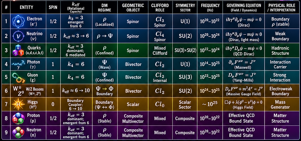
These values count the number of independent relational planes available in each dimensional sector. In the table, k_eff denotes the dominant accessible relational plane count of the particle’s governing regime. For localized matter, the dominant sector is typically 3D. For propagating gauge fields, the dominant sector is 4D. For coherence-transition or boundary-active states, the capacity is written as a crossover such as 3 → 6 or 6 → 10.
Table Notes
• Relational capacity is assigned by governing geometric sector, not treated as a standalone intrinsic particle constant.
• The notation 3 → 6 indicates transition between localized matter structure and propagating spacetime plane structure.
• The notation 6 → 10 indicates transition between 4D plane structure and 5D coherence-boundary structure.
• For composite baryons such as the proton and neutron, k_eff is listed as 3 dominant because the stable observable state is localized, while the internal gauge dynamics still require 4D mediation.
• The Higgs is scalar by spin grade but is listed as a boundary coupler because its role is to mediate sectoral transition rather than act as a propagating bivector field.
Standard Model states are not only classified by spin and symmetry, but also by the effective number of independent geometric relations accessible in their dominant dimensional regime. This turns the table into a unified map connecting representation theory, Clifford geometry, DM regimes, and structural capacity.
Note:
Why spin is naturally associated with geometric grade in Clifford algebra.
In spacetime, the infinitesimal generators of rotations and boosts are bivectors, represented by the antisymmetric commutators of gamma matrices. Spin therefore describes how states transform under bivector plane rotations. Spinors are naturally represented in the even subalgebra of the Clifford algebra, which explains both their geometric role and the characteristic 4π rotation property of spin-1/2 systems.
Geometrically, a rotation occurs in a plane. In Clifford algebra, planes are represented by bivectors. This is the first reason spin is tied to geometric grade.
rotation ⇄ plane ⇄ bivector [Spin is plane-rotation geometry.]
In relativistic quantum theory, the generators of infinitesimal Lorentz transformations acting on spinor fields are
Σ^{μν} = (i/2)[γ^μ, γ^ν]
The commutator is antisymmetric in μ and ν, so each generator corresponds to a spacetime plane. These are precisely the bivector generators of the spacetime Clifford algebra. [The Lorentz generators are antisymmetric plane generators, i.e. bivectors.]
Counting Independent Planes
The number of independent planes in n dimensions is
kₙ = n(n - 1) / 2
For spacetime with n = 4, this gives
k₄ = 4(4 - 1) / 2 = 6
So 4D spacetime contains six independent planes. These correspond to the six independent components of Σ^{μν}: three spatial rotations and three boosts. [k₄ = 6 matches the six independent Lorentz bivector generators.]
Why Spinors Belong to the Even Subalgebra
Spinors are naturally generated by products of an even number of vectors. In Clifford algebra, the even subalgebra contains scalars, bivectors, and higher even-grade elements. Since rotations are generated by bivectors, spinor transformations are built from exponentials of bivectors.
R = exp(-B θ / 2) Here B is a bivector specifying the plane of rotation. A spinor state ψ transforms under the rotor R as ψ' = R ψ
This is why spinors encode orientation across planes rather than ordinary vector direction. [Spinors live in the even Clifford structure because rotations are generated by bivectors.]
Why Spin-1/2 Has 4π Symmetry
Because the spinor transformation uses a half-angle in the rotor exponential, a 2π spatial rotation changes the sign of the spinor rather than returning it to its original value.
R(2π) = exp(-Bπ) = -1
Only after a full 4π rotation does the spinor return to its original state:
R(4π) = exp(-B2π) = +1
This explains the characteristic double-cover behavior of spin-1/2 representations. [The 4π property follows from bivector-generated half-angle spinor rotations.]
The chain of reasoning is therefore direct. Rotations occur in planes. Planes are bivectors. The generators of spin transformations in spacetime are the antisymmetric bivector operators Σ^{μν}. The number of such independent plane generators is k₄ = 6 in four dimensions. Spinors transform under exponentials of these bivectors and therefore belong naturally to the even Clifford subalgebra. For this reason, spin is most naturally understood as bivector geometry rather than as literal spinning in three-dimensional space.
[Spin ⇒ plane rotations ⇒ bivectors ⇒ even Clifford algebra.]
Dimensional Clarity with DM
1. Dimension – hierarchical extension (0D → 5D):
Penteract → Tesseract → Cube → Square → Line → Point
Each dimension completely contains the previous. Every face is a lower dimensional boundary. Information is always stored on faces. Reduction chain:
• Φ (5D coherence)
• Ψ (4D wavefunction)
• ρ (3D observers)
• ⟂ (2D cross-section)
Time evolution contains spatial localization (t↑ - m↓).
Collapse of t-axis: ρ(t₀) = ∫ Ψ δ(t−t₀) dt = Ψ(t₀) (10¹²¹ → 10⁶¹) B₄ → B₃
Global correlation contains temporal evolution (m↑ - t↓).
Collapse of s-axis: Ψ = ∫₀^∞ Φ e^(−s/λₛ) ds = Φ λₛ (10¹²² → 10¹²¹) B₅ → B₄
2. Boundary Projection– each dimension is defined by its lower-dimensional surface because higher-dimensional information reduces to lower-dimensional observations:
• ∂Mⁿ = Mⁿ⁻¹
Interactions occur across boundaries. (Hint: humans only perceive 2D boundaries of 3D objects.)
• Entropy arises from boundary counting
S ∝ Area.
Derived from number of 2D planes in higher-dimensional structure
3. Cross-Section – observable structures arise as slices of higher-dimensional objects
• ρ(x, y, z) = ∫ Ψ(x, y, z, t) δ(t − t₀) dt = Ψ(x, y, z, t₀)
Quantum measurement corresponds to cross-sectional extraction (4D → 3D).
• Coxeter Plane counts (cross-section counting):
kₙ = n(n−1)/2k₂=1, k₃=3, k₄=6, k₅=10. These determine reflection symmetries, orbital capacities, and scaling behavior.
Particle masses cluster at 10²³–10²⁵ Hz. The electron rest-frequency (~10²⁰ Hz) marks the transition between orbital and particle regimes, while fusion is the geometric transition.
4. Closure – stable structures arise from closed geometric cycles
• Particles → closed reflection orbits
• Atoms → closed orbital structures
• Fields → continuous closure in spacetime
Open structures correspond to unstable or confined states.
5. All scaling laws arise from projection depth
ƒ(s) = ƒₚ e^(−s/λₛ) generates: particle masses, frequency bands and cosmological scaling
Constants emerge as invariants of this structure. A ladder from biological rhythms (Hz) to qubits (GHz), to Particle masses cluster at 10²³–10²⁵ Hz, to the Higgs, and up to the Planck frequency (~10⁴³ Hz). The electron rest-frequency (~10²⁰ Hz) marks the transition between orbital and particle regimes, while fusion is the geometric transition.
• The sequence B₃ → B₄ → B₅ precisely maps to the evolution of localized matter (ρ), time (Ψ), and coherence (Φ), corresponding respectively to classical physics, wave–spacetime, and coherence-stabilized fields.
• The Coxeter Bₙ sequence defines the discrete reflection symmetries underlying reality’s geometry. Each dimensional expansion adds an orthogonal axis of movement.
Black Holes and Quantum Computing
This section provides a mathematical explanation of the deep connection between black holes and quantum computing, focusing on three correspondences: boundaries, entropy, and information capacity.
Event Horizon ⇄ Qubit Boundary
Black hole entropy:
S_BH = (k_B A) / (4 ℓₚ²)
A black hole’s event horizon acts as a boundary that separates what can and cannot be observed. All information about the black hole is encoded on this surface.
Open quantum system:
dρ/dt = -i/ħ [H, ρ] + L_env(ρ)
In a quantum computer, the qubit boundary plays a similar role. It defines how well the system is isolated from its environment. A strong, well-controlled boundary preserves quantum information, while a weak boundary allows information to leak out.
In both cases, the boundary determines how information is stored and whether it remains accessible.
Entropy ⇄ Decoherence Rate
Entropy:
S = -k_B Tr(ρ ln ρ)
Entropy in a black hole measures how much information is hidden or compressed. A black hole represents a system with extremely high entropy, meaning information is maximally packed.
Decoherence:
ρᵢⱼ(t) = ρᵢⱼ(0) e^{-Γ t}
In quantum computing, decoherence measures how quickly information is lost from a quantum state. As decoherence increases, the system behaves more classically and loses its quantum properties.
These two concepts are closely related. Increasing entropy corresponds to a loss of structured information, which is the same effect seen when decoherence destroys quantum coherence. As entropy increases, coherence decreases:
dS/dt ∝ Γ
Area Law ⇄ Error Correction Capacity
Black hole area law:
S ∝ A
In black holes, the amount of information that can be stored is proportional to the surface area of the event horizon. This is known as the area law.
Entanglement entropy:
S_A ∼ |∂A|
Quantum error correction:
|ψ_L⟩ = Σ cᵢ |codeᵢ⟩
In quantum computing, error correction works by distributing information across many physical qubits. The more structure and connectivity the system has, the more robust it becomes against errors.
Both systems show that information protection depends on how it is distributed across boundaries rather than how much volume is available.
Unified Interpretation
S ∼ ∫_{∂M} dA / ℓₚ²
dρ/dt = -i/ħ [H, ρ] - Γ(∂M) ρ
Boundary geometry controls entropy, decoherence, and information capacity.
These relationships reveal a deeper principle: information in physical systems is governed by geometry. Boundaries determine what information is accessible, entropy describes how information is distributed, and structure determines how well that information can be protected.
Black holes represent a natural system where information is maximally stabilized, while quantum computers are engineered systems that attempt to preserve that same kind of stability under controlled conditions.
Black holes and quantum computers are both systems of geometric information.

Constants Organized
Speed of light c
c ≈ 2.99792458 × 10⁸ m/s
c = λ ƒ
ℓₚ = c tₚ
c = ℓₚ ƒₚ
The kinematic invariant relating spatial update to scan rate.
Planck constant h
h ≈ 6.62607015 × 10⁻³⁴ J·s
E = h ƒ
h = Eₚ tₚ
The action quantum linking frequency to energy.
Reduced Planck constant ħ
ħ = h / (2π)
ψ = √ρ e^(iS/ħ)
m(s) t(s) = ħ / c²
The phase-normalization constant that appears in rotational and wave dynamics. It is the natural angular/rotational normalization of the scan-action relation.
Gravitational constant G
G ≈ 6.67430 × 10⁻¹¹ m³ kg⁻¹ s⁻²
ℓₚ = √(ħG/c³)
tₚ = √(ħG/c⁵)
mₚ = √(ħc/G)
The coupling constant between mass-energy and curvature.
Planck length ℓₚ
ℓₚ ≈ 1.616255 × 10⁻³⁵ m
ℓₚ = √(ħG/c³)
ℓₚ = c / ƒₚ
The minimal spatial resolution.
Planck time tₚ
tₚ ≈ 5.391247 × 10⁻⁴⁴ s
tₚ = √(ħG/c⁵)
ƒₚ = 1 / tₚ
The minimal temporal resolution.
Planck frequency ƒₚ
ƒₚ ≈ 1.85 × 10^43 Hz
ƒₚ = 1/tₚ
f(s) = fₚ e^(-s/λₛ)
The UV anchor of the full coherence ladder.
Planck mass mₚ
mₚ ≈ 2.176434 × 10⁻⁸ kg
mₚ = √(ħc/G)
mₚ = h fₚ / c²
The natural mass associated with a maximally localized Planck-frequency mode.
Hubble constant H₀
H₀ ≈ 2.2 × 10⁻¹⁸ s⁻¹
H₀ = fₚ e^(-s_H/λₛ)
(ƒₚ / H₀) ≈ 10⁶¹
(ƒₚ / H₀)² ≈ 10¹²²
The cosmological IR scan rate. The extreme low-frequency endpoint reached by coherence-axis projection.
Fine-structure constant α
α ≈ 1/137
α = e² / (4π ε₀ ħ c)
The effective participation ratio of electromagnetic plane-harmonic organization to total symmetry capacity.
Boltzmann constant k_B
k_B ≈ 1.380649 × 10⁻²³ J/K
k_B T
k_B T(s) t(s) = h
The conversion between temperature and energy. It sets thermal excitation strength for plane-harmonic modes.
Cosmological constant Λ
Λ ~ 10⁻⁵² m⁻²
Λ ~ H₀² / c²
The vacuum curvature scale. A residual IR curvature left after coherence-axis projection.
Coherence length λₛ
model parameter
ƒ(s) = ƒₚ e^(-s/λₛ)
R(s) = ℓₚ e^(+s/λₛ)
The decay/expansion scale along the coherence axis.
Relational capacity kₙ
kₙ = n(n−1)/2
k₃ = 3
k₄ = 6
k₅ = 10
The number of independent relational planes or pairwise channels in n dimensions. It is the maximum local channel count available to geometry, fields, and decoherence.
Symmetry capacity |Bₙ|
|Bₙ| = 2ⁿ n!
|B₃| = 48
|B₄| = 384
|B₅| = 3840
The size of the hypercubic Coxeter symmetry group of the sector. It measures orientation, reflection, and permutation capacity.
Mode capacity Nₙ
Nₙ = ηₙ |Bₙ|
0 ≤ ηₙ ≤ 1
The physically occupied fraction of the total symmetry orbit. It measures how much of the sector’s total mode capacity is actually realized.
Rather than treating constants as independent inputs, here, they are derived as invariants of a geometric scan structure connecting M³ (cube), M⁴ (tesseract), and M⁵ (penteract) regimes. The Planck scale defines the ultraviolet (UV) anchor of this structure, while the Hubble scale defines its infrared (IR) endpoint.
The Planck scale defines a universal scan interface, and all physical constants emerge as relations preserved under projection along x,y,z, x,y,z,t, and x,y,z,t,s axes. Constants such as c, h, G, and H₀ are geometric invariants governing transformations between frequency, space, time, energy, and curvature.
The hierarchy between Planck and cosmological scales naturally generates the relation (fₚ / H₀)² ~ 10¹²², providing a geometric explanation for the cosmological constant problem.
Discrete geometric structures—captured by relational capacity kₙ = n(n−1)/2 and Coxeter symmetry |Bₙ| = 2ⁿ n!—define the available mode and symmetry capacity of physical systems. Therefore, observable physics directly arises from the projection and truncation of these capacities into lower-dimensional regimes.
All constants of nature can be organized into three interconnected classes.
1. Scan invariants (c, h, ℓₚ, tₚ, ƒₚ): These define the fundamental resolution and update rules of the
geometric scan.
2. Coherence invariants (H₀, λₛ, Λ): These govern how high-frequency Planck-scale structure projects into observable low-frequency regimes.
3. Symmetry invariants (kₙ, |Bₙ|, Nₙ): These define the relational and symmetry capacity available to
physical systems.
Together, these constants form a closed system of relations derived from geometry, frequency scaling, and coherence projection. The framework suggests that physical law is not fundamentally dynamical-first, but geometry-first, with algebraic dynamics emerging as a secondary description of underlying geometric structure.
The DM framework implies:
• Physical laws are geometric projections
• Quantum and gravitational phenomena are unified through coherence
• Particle physics emerges from symmetry and mode capacity
This shifts physics from a dynamics-first paradigm to a geometry-first paradigm.
1 Dynamics → change along axes: n → degrees of freedom
2 Interactions → pairwise relations: kₙ = n(n−1)/2
3 Observability → boundary projection: dim(∂Mᴰ) = D−1
4 State space → symmetry structure: |Bₙ| = 2ⁿ n!
Static vs Dynamic View
The Planck Scan is Dimensional Analysis extended into a continuous trajectory along the coherence axis.
Dimensional Analysis (standard)
[Q] = [L]ᵃ [T]ᵇ [M]ᶜ
Planck Scan
Q(s) = Qₚ e^(±s/λₛ)
• same dimensional structure
• but now evolving along the s-axis
All dimensional constraints remain intact:
Energy–frequency
E = h ƒ
Light-speed relation
c = λ ƒ
Mass–energy
E = m c²
Planck closure
ℓₚ = √(ħ G/c³)
Distance along the s-axis
ƒₚ / H₀ ~ 10⁶¹
• UV (Planck) → s = 0
• IR (cosmic) → s ~ 61 λₛ
The simplest diagonal metric reproduces the exponential ladder, while curvature in coupling directions generates geometric beta-functions. Dependence of the spacetime metric on the coherence coordinate produces an Einstein correction tensor from ∂ₛ-gradients. LHC mass bands, decoherence rates, and cosmological expansion then appear as ultraviolet, intermediate, and infrared observables of one common geodesic structure.
UV/IR hierarchy and the cosmological 10¹²² scale
Relation between the Planck scan rate and the cosmological expansion rate.
ƒₚ / H₀ ≈ 10⁶¹
(ƒₚ / H₀)² ≈ 10¹²²
The unsquared ratio is the UV/IR scan-depth hierarchy. The squared ratio is the area/curvature hierarchy, and it naturally matches the famous 10¹²² cosmological hierarchy associated with vacuum-energy and horizon-scale comparisons.
Frequency ladder relations
Once a frequency is selected, all major dimensional quantities follow from a one-parameter ladder:
t = 1/ƒ
E = h ƒ
m = h ƒ / c²
λ = c / ƒ
κ = 1/λ² = ƒ² / c²
This is why the constants c and h are so central in the framework: they transmit the frequency choice into all other observable scales.
Coherence ladder relations
ƒ(s) = ƒₚ e^(-s/λₛ)
E(s) = Eₚ e^(-s/λₛ)
m(s) = mₚ e^(-s/λₛ)
R(s) = ℓₚ e^(+s/λₛ)
t(s) = tₚ e^(+s/λₛ)
These relations show how the constants anchor both the UV endpoint and the observable low-frequency projection of the ladder.
Taken together, these constants form a coupled system rather than a disconnected list. In DM, c fixes the scan speed, h fixes the action per scan, G fixes the curvature response, ℓₚ–tₚ–ƒₚ fix the UV interface, H₀ fixes the IR endpoint, λₛ fixes the projection depth scale, and kₙ–|Bₙ|–Nₙ fix the geometric and symmetry capacity of each sector.
Prediction: Increased effective coherence depth s leads to measurable extension of coherence time.
Γ_DM = Γ₀ e^{-β s/λₛ}
T₂ ∝ e^{+β s/λₛ}
Operational
s_eff = λₛ ln(T₂ / T₂,₀)
Unit Identity: SI–Planck
This section unifies SI units, Planck units, dimensional closure, and coherence scaling into one statement. Planck units define the intrinsic structural anchors, while physical constants act as closure operators that map human-scale SI measurement onto geometric reality. Physics already connects SI and Planck units numerically – but not structurally.
1. Full observable unit form
[Q] = [L]ᵃ [M]ᵇ [T]ᶜ [I]ᵈ [Θ]ᵉ [N]ᶠ [J]ᵍ [S]ʰ
This is the most general dimensional form used in DM once the coherence axis [S] is added to the ordinary SI basis.
2. Minimal structural basis
DM minimal basis = {[L], [T], [M], [S]}
The first reduction step is the SI Reduction Theorem: the independent structural basis is not the full SI set, but the smaller geometric basis {L, T, M, S}. Current, temperature, amount of substance, and luminous intensity are derived measurement-level quantities.
3. Closure operators
c: [L][T]⁻¹
ħ: [M][L]²[T]⁻¹
G: [L]³[M]⁻¹[T]⁻²
k_B: [M][L]²[T]⁻²[Θ]⁻¹
e: [I][T]
These constants are interpreted not as arbitrary inserted numbers, but as closure operators. They enforce consistent relations between otherwise independent axes.
c: space ⇄ time, ħ: energy ⇄ frequency, G: mass ⇄ curvature
4. Planck anchors
ℓₚ = √(ħG / c³)
tₚ = √(ħG / c⁵)
mₚ = √(ħc / G)
Tₚ = √(ħc⁵ / (G k_B²))
Planck quantities arise as the intrinsic intersection point of closure operators. They therefore anchor the structural layer.
• SI (meters, seconds, kg): the measurement layer (what we read on instruments).
• Planck (ℓₚ, tₚ, mₚ): the structural layer (how reality is built).
5. Collapse identity
[Q] → [L]ᵃ [M]ᵇ [T]ᶜ [S]ᵈ
[Q] → ℓₚᵃ mₚᵇ tₚᶜ Sᵈ
Once closure is imposed, the observable unit system collapses into powers of geometric anchors. The apparent multiplicity of units is reduced to a smaller structural core.
6. Scaling identity
R(s) = ℓₚ e^(s/λₛ)
ƒ(s) = ƒₚ e^(-s/λₛ)
R(s) ƒ(s) = c
The unit system is not static. Through the coherence coordinate s, every measurable quantity sits on a continuous ladder between Planck structure and SI-scale observables.
Units = projected coordinates on a dimensionally closed geometric system
Constants = closure operators
Planck units = structural anchors
SI units = observer-scale projections
7. Compact form
{SI} + {c, ħ, G, k_B, e} + {Planck anchors} = one closed geometric system
Measurement → closure → geometry
SI and Planck do not describe separate realities. They are two coordinate descriptions of the same dimensionally closed structure.
Plain language
• Units are labels, not the thing itself.
• Constants are conversion rules between labels.
• Planck units are the native 'grid' of reality.
• SI units are how observers read that grid.
• Put together, physics becomes a single geometric system.
This removes arbitrariness from constants, simplifies equations, and provides a direct path to engineering, by working with structure (geometry) instead of labels (units).

Subjective Mass
~10¹²²
S = ∇ₛ² Φ - Λₛ e^(-s/λₛ)
Objective Identity
"Length" no longer applies in the classical sense?
(ρ) (Ψ) (Φ)
Dimensional Memorandum
T' = T · √(1 – v²/c²)
x, y, z, t, s
Activation Threshold
~10³³-10⁴³ Hz
Ψ
astrophysical phenomena
Orientation
Originated 2023, Presented 2025
Author: J. Theders
biological quantum systems
Ψ
Φ
10²⁵ Hz
10³³-10⁴³
10⁴³
mₙ = Eₚ · e^(–n / λₛ)
Γeff = Γ₀ e^(–s / λₛ)
Φ
energy thresholds (Eₚ)
Physical Laws
Geometry 101
10¹⁵ Hz
Particles below this threshold
Where is Space?
When is Time?
(c = lₚ / tₚ)
Mass = Localized wave without time (t)
s-depth: s ≈ 0.8–4.0
𝓘ₙ = ∑(Tᵢ + T̄ᵢ) · e^(–s / λₛ)
𝓛DM = (c⁴ / 16πG)(R + S) + 𝓛ρ + 𝓛Ψ + 𝓛Φ
Ψ(x,y,z,t) = ∫ Φ(x,y,z,t,s) · e^(−s/λₛ) ds
ρ(x,y,z; t₀) = ∫ Ψ(x,y,z,t) · δ(t−t₀) dt
Here λₛ represents coherence depth, and δ(t−t₀) defines the instantaneous 3D observational slice. Thus, the wavefunction Ψ is not just information—it is a 4D structure stabilized by Φ.
Humans are not separate from the information they generate. Just as the wavefunction is real coherence, the 'self' is coherence stabilized across ρ, Ψ, and Φ. This reframes both quantum mechanics and consciousness as parallel manifestations of nested geometry.
1) Wavefunction projection:
Ψ(x,y,z,t) = ∫ Φ(x,y,z,t,s) · e^(−s/λₛ) ds
2) Observed state:
ρ_obs(x,y,z; t₀) = ∫ Ψ(x,y,z,t) · δ(t−t₀) dt
3) Born’s rule (as projection measure):
p_i = |⟨e_i|Ψ⟩|² = overlap measure of Ψ with ρ-subspace.
4) Identity stabilization:
I = ∫ Ψ_neural(x,t) · e^(−s/λₛ) ds
Both particles and human beings are coherence-stabilized information structures.
c = R(s)·ƒ(s)
Wavefunction Collapse
Standard physics describes collapse mathematically but does not explain why measurement irreversibly destroys superposition. The invariant c = R(s)·ƒ(s) shows collapse is dimensional exhaustion: when R expands (localization), ƒ contracts (phase lost).
Why Entanglement Appears Nonlocal
Nonlocality violates no geometry once distance R is traded against frequency ƒ along s. Entangled systems share high-ƒ coherence even when R is large.
Why Gravity Resists Quantization
Gravity operates where R is maximized and ƒ minimized, making discrete quanta inaccessible. Quantization fails because gravity is a coherence-gradient, not a particle exchange.
Origin of the Speed of Light
c is not a fundamental speed but the invariant exchange rate between spatial extension and frequency compression.
Why Mass Has Rest Energy mc²
Mass is frozen phase. Rest energy emerges from the balance point where time and frequency convert geometrically.
Why Time Has an Arrow
As s increases, ƒ decreases monotonically while R increases, enforcing irreversibility without entropy postulates.
Why the Vacuum Has Structure
Vacuum energy is residual high-ƒ coherence after R expansion, explaining Casimir forces and dark energy scaling.
Why Chemistry Stops at the Electron
At the electron Compton frequency, 3D localization saturates; above this ƒ regime chemistry dissolves into relativistic coherence.
Why Black Hole Entropy Scales with Area
Only transverse faces of higher-dimensional coherence project into 3D, enforcing area—not volume—entropy.
Why There Are Dimensional Phase Boundaries
The c-ladder (sub-c¹ to c⁵) corresponds to how many orthogonal axes contribute to propagation; phase transitions are geometric.
Why Measurement Destroys Qubits
Reading forces R↑ and ƒ↓, eliminating phase degrees of freedom required for quantum computation.
Why the Cosmological Constant Is Small
Λ is suppressed by exponential ƒ decay along s while R inflates, naturally yielding the 10¹²² gap.
Why Classical Reality Exists At All
Classicality is the low-ƒ, high-R limit of the same invariant, not a separate regime.
Why This Produces Quantum “Weirdness”
(A) Superposition
Ψ = Σᵢ cᵢ ψᵢ
ρ = |Ψ|²
Multiple higher-dimensional components project onto a single boundary slice.
Result: Appears as “many states at once.”
(B) Collapse
ρ(t₀) = ∫ Ψ(x,y,z,t) δ(t - t₀) dt
You are slicing along the time axis.
Result: A continuous structure appears to “collapse.”
(C) Entanglement
Ψ(x₁, x₂, t)
ρ(x₁, x₂)
Correlation exists in higher dimension—projection preserves it instantly.
Result: Appears “nonlocal.”
Quantum mechanics is what a higher-dimensional geometric structure looks like when observed through a lower-dimensional boundary.


Ψ(x, y, z, t)
Wavefunction
ρ(x, y, z)
Local
⟂( y, z)
Cross-section
Φ(x, y, z, t, s)
Coherence Field


1D
2D
3D
4D
0D
5D
(x)
(x, y)
(x, y, z)
(x, y, z, t)
Geometry to Cosmology
1. Geometric Foundation
kₙ = n(n−1)/2
Defines relational planes and geometric structure.
2. Symmetry Structure
|Bₙ| = 2ⁿ n!
Defines full symmetry orbit of configurations.
3. Mode Capacity
Nₙ = kₙ × 2 × 2 × 4
Total available plane-harmonic modes.
4. Occupancy
ηₙ = N_active / |Bₙ|
Fraction of occupied relational capacity.
5. Frequency Mapping
E = h ƒ
ƒ(s) = ƒₚ e^{-s/λₛ}
Positions systems along coherence ladder.
6. Atomic Structure
Orbitals correspond to frequency bands; periodic table is mode filling.
7. Chemical Bonding
ψ = Σ Aᵢⱼ e^{iθᵢⱼ}
Bonding arises from plane coupling.
8. Relational Density
ρ_rel = ηₙ |Bₙ|
Effective density of occupied structure.
9. Projection to Physics
T_{μν} = Π_{μν}[ρ_rel]
Relational density becomes energy-momentum.
10. Einstein Closure
G_{μν} = (8πG/c^4) T_{μν}
Curvature emerges from relational structure.
11. Nuclear Decay
ηₙ > η_stable ⇒ emission
Local coherence relaxation.
12. Black Hole Radiation
T_H = ħ c³ / (8π G M k_B)
Horizon-scale relaxation.
13. Cosmic Expansion
H² = (8πG/3)ρ + Λ/3
Global relaxation.
14. Unified Law
Δρ_rel < 0
Physics = geometry × symmetry × occupancy × relaxation
Variational Selection Principle
δ[∫ ρ(∂t S + (∇S)²/(2m) + V) + λ ∫ (∇ρ)²/ρ + η A/ℓₚ²] = 0
Balances dynamics, information, and geometry.
Projection
ψ = ∫ Φ e^{-s/λₛ} ds
ρ = |ψ|²
Selection → Projection → Observable
Evolution
Schrödinger: iħ ∂ψ/∂t = Hψ
Lindblad: dρ/dt = -i/ħ[H,ρ] + Σ(LρL† - ½{L†L,ρ})
Physical reality is a boundary-constrained, information-geometric, plane-harmonic system selected variationally, projected by coherence, organized by symmetry, scaled by frequency, and evolved via quantum and open-system dynamics.